The Hyperbolic setting¶

Invariant sets (see Definition here) play a fundamental role in dynamical systems theory. In particular, they cannot be “crossed” by trajectories and therefore they play a role in determining the possibilities for how trajectories may navigate phase space, i.e. phase space transport. Invariant sets can be characterized by their stability properties. Further, these can be divided into stability characteristics normal to the invariant set and tangential to the invariant set. The normal stability properties indicate how trajectories near, but not contained in, the invariant set behave.

Normally hyperbolic invariant sets play a particularly important role in phase space transport, particularly when the invariant set has the additional property of being an invariant manifold. For our purposes the reader can think of an invariant manifold as being a generalization of a curve or surface for which the equation defining such a mathematical object is differentiable [GP10]. Normally hyperbolic invariant manifolds (NHIMs) have invariant stable and unstable manifolds that form the skeleton or framework, on which phase space transport occurs. But before we discuss normally hyperbolic invariant manifolds in general, we discuss the simplest type of non-trivial type of normally hyperbolic invariant manifold—a hyperbolic periodic orbit.

Unstable periodic orbits play an important role in our understanding of the dynamics of Hamiltonian systems. Periodic orbits have constant energy, as well as their stable and unstable manifolds, and are contained in the energy surface that is of one less dimension than the dimension of the phase space, i.e. the energy surface has codimension one. In general, the codimension of a surface contained in phase space is the dimension of phase space minus the dimension of the surface. If the codimension is one then it may divide the ambient space, and therefore act as a barrier to transport in the space.

In two degree-of-freedom Hamiltonian systems a one dimensional unstable periodic orbits has two dimensional stable and unstable manifolds that can “divide” the energy surface and can be used to create invariant regions (“lobes”) that transport throughout the phase space, while respecting the “barrier nature” of invariant manifolds.

For more than two degrees-of-freedom periodic orbits and their stable and unstable manifolds do not have sufficient dimension (or, equivalently, their codimension is greater than one) to form barriers to transport or lobes.

We also note (cf. Section 3 ) the global phase space structure can be studied by creating a mapping along trajectories from a surface transverse to the flow in the energy surface, i.e. the Poincaré map and the Poincaré section. For two degrees-of-freedom the Poincaré section is two dimensional. For \(n\) degrees-of-freedom the Poincaré section is \(2n-2\) dimensional. The dynamics in the Poincaré section is not easy to visualize for more than two degrees-of-freedom.

In the table below we collect together some dimensionality and codimensionality properties of periodic orbits and their associated geometrical structures within the energy surface, i.e. \(E= {\rm constant}\).

Table 1 Dimension count of phase space structures. Codimension of certain objects appears in parentheses.¶
Degrees of freedom	2	3	\(n\)
Phase space	4	6	\(2n\)
Energy surface	3	5	\(2n\)
Poincaré section	2	4	\(2n-2\)
Periodic orbit	1 (2)	1 (4)	1 (\(2n-2\))
Stable and unstable manifolds of a periodic orbit	2 (1)	2 or 3 (3 or 2)	2 to \(n\) (\(2n-3\) to \(n-1\))
Barriers in energy surface	2 (1)	4 (1)	\(2n-2\) (1)

NHIMs are a generalization of unstable periodic orbits to more than two degrees-of-freedom in this sense that they may have stable and unstable manifolds of codimension one in the energy surface and, hence, for the framework on which phase space transport occurs in Hamiltonian systems with more than two degrees-of-freedom [Wig90]. Now we want to develop this idea of a NHIM, and its consequences, in more detail. Recent references for this topic are [Wig94][WWJaffeU01][Wig04][Eld13], but we will begin with an elementary description.

In understanding what is meant by “normally hyperbolic invariant manifold” we start by explaining the last word in the phrase and working towards the first.

A manifold is the natural generalization of a differentiable curve or surface.
A set in the constant energy level set is called invariant under the flow if any trajectory in the set is contained in the set at all times (link to definition in previous chapter).
Normal hyperbolicity means that locally under the linearized dynamics, the growth and decay rates in the normal directions to the manifold dominate the growth and decay rates tangent to it. These growth rates are quantified by eigenvalues of the matrix associated with the linearization for equilibria, Floquet exponents for the monodromy matrix associated with periodic orbits, and generalized Lyapunov exponents for more general invariant manifolds [Fen71].

Now we consider a number of simple examples in order to explain in more detail these concepts. The following exposition is based on the works [WWJaffeU01][Wig16b].

In all of our examples in this section we will consider the classical autonomous Hamiltonian obtained as the sum of kinetic plus potential energy \((H = K + V)\).

One Degree-of-Freedom Hyperbolic Equilibrium Point¶

The most simple Hamiltonian function with a hyperbolic equilibrium point is

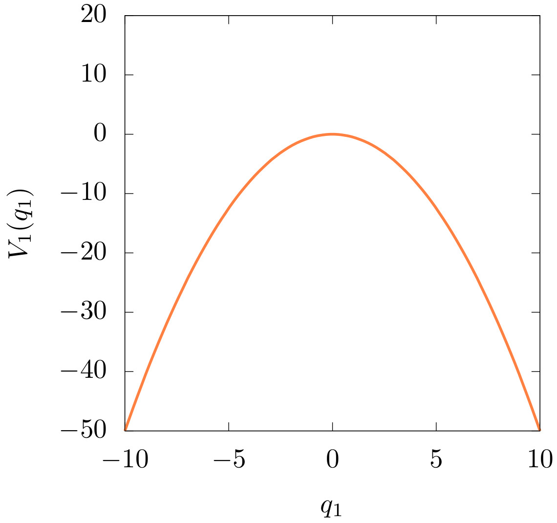
(19)¶\[\begin{equation} H = K_{1}(p_{1}) + V_{1}(q_{1})= \frac{\lambda}{2} (p^2_1 - q^2_1) ,\quad \lambda > 0, \end{equation}\]

Fig. 1 The potential energy \(V(q_1)\). An unstable equilibrium point is located at \(q_1=0\).¶

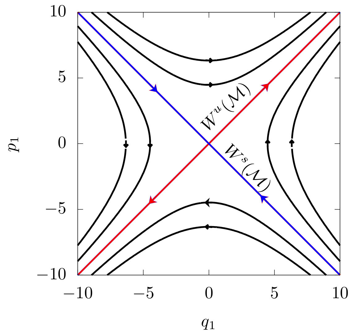
Fig. 2 Plane \(q_1\)–\(p_1\). The equilibrium point is at the origin \(\mathcal{M}=(q_1=0, p_1=0)\). The red line is the stable manifold \(W^s(M)\), the blue line is the unstable manifold \(W^u(M)\).¶

The equations of motion are

(20)¶\[\begin{split}\begin{eqnarray} \dot{q_1} &=& \frac{\partial H}{ \partial p_1} =\lambda p_1 \nonumber \\ \dot{p_1} &=& -\frac{\partial H}{ \partial q_1} = \lambda q_1. \end{eqnarray}\end{split}\]

For energies \(E_1<0\) the energy level set consists of two disconnected parts, a trajectory cannot reach \(q_1=0\) due insufficient energy. For \(E_1=0\) the two previously disconnected parts connect at \(q_1=p_1=0\) and for energies \(E_1>0\), any value of \(q_1\) is accessible.

The origin, \(\mathcal{M} = (q_1=0,p_1=0)\), is a equilibrium point of the system. The trajectory that starts at \(\mathcal{M}\) remains always at the same point.

Showing the invariance of candidate sets.

Let us consider the line \(q_1 = - p_1\). The Hamiltonian vector field evaluated on the line is tangent to the line.

(21)¶\[\begin{split}\begin{eqnarray} \dot{q_1} &=& -\lambda q_1 \nonumber \\ \dot{p_1} &=& -\lambda p_1. \label{eq:ws} \end{eqnarray}\end{split}\]

A trajectory that starts on the line \(q_1 = - p_1\) remains on the line. This line is an invariant set under the flow.

The solution of the system of differential Eq. (21) decay exponentially in time.

(22)¶\[\begin{split}\begin{eqnarray} q_1(t) &=& q_1(0) e^{-\lambda t} \nonumber\\ p_1(t) &=& p_1(0) e^{-\lambda t}. \end{eqnarray}\end{split}\]

Any trajectory that starts on \(q_1 = - p_1\) converges to the equilibrium point \(\mathcal{M}\) in an infinite time. These properties motivate the definition of the stable manifold of the set \(\mathcal{M}\). The stable manifold \(W^s(\mathcal{M})\) of the set \(\mathcal{M}\) is the set of points in the energy level set such that their corresponding trajectories converge to the set \(\mathcal{M}\) when the time goes to infinity.

(23)¶\[\begin{equation} \displaystyle{ W^s(\mathcal{M})= \lbrace (q_1,p_1) | (q_1(t), p_1(t) ) \rightarrow \mathcal{M} , t \rightarrow + \infty \rbrace} = \lbrace (q_1, p_1 ) | q_1 = - p_1 \rbrace \end{equation}\]

Now, let us consider the trajectories that start on the line \(q_1 = p_1\). Like in the previous case, the Hamiltonian vector field is tangent to the line,

(24)¶\[\begin{split}\begin{eqnarray} \dot{q_1} &=& \lambda q_1 \nonumber\\ \dot{p_1} &=& \lambda p_1. \end{eqnarray}\end{split}\]

However, the vector field points away from \(\mathcal{M}\). The trajectories that start on the line \(q_1 = p_1\) diverge from the equilibrium point \(\mathcal{M}\).

(25)¶\[\begin{split}\begin{eqnarray} q_1(t) &=& q_1(0) e^{\lambda t} \nonumber\\ p_1(t) &=& p_1(0) e^{\lambda t}. \end{eqnarray}\end{split}\]

Analogously, these properties motivate the definition of the unstable manifold of the set \(\mathcal{M}\). The unstable manifold \(W^u(\mathcal{M})\) of \(\mathcal{M}\) is the set of points in the phase space such that their corresponding trajectories converge to the set \(\mathcal{M}\) when the time goes to minus infinity.

(26)¶\[\begin{equation} \displaystyle{ W^u(\mathcal{M})= \lbrace (q_1,p_1) | (q_1(t), p_1(t) ) \rightarrow \mathcal{M} , t \rightarrow - \infty \rbrace = \lbrace (q_1, p_1 ) | q_1 = p_1 \rbrace }. \end{equation}\]

The existence of two special directions where the trajectories converge to the \(\mathcal{M}\) in some direction and diverge from \(\mathcal{M}\) in other one is the essence of the concept of hyperbolicity.

Two Degrees-of-Freedom and the Hyperbolic Periodic Orbit¶

In this case, the Hamiltonian function for the 2-degree of freedom system is the sum of the Hamiltonian function of the 1-degree of freedom of the previous example plus the Hamiltonian of a harmonic oscillator (Section An Informal Introduction to Ideas Related to KAM (Kolmogorov-Arnold-Moser) Theory ). The total energy of the system is split between both DoF to yield:

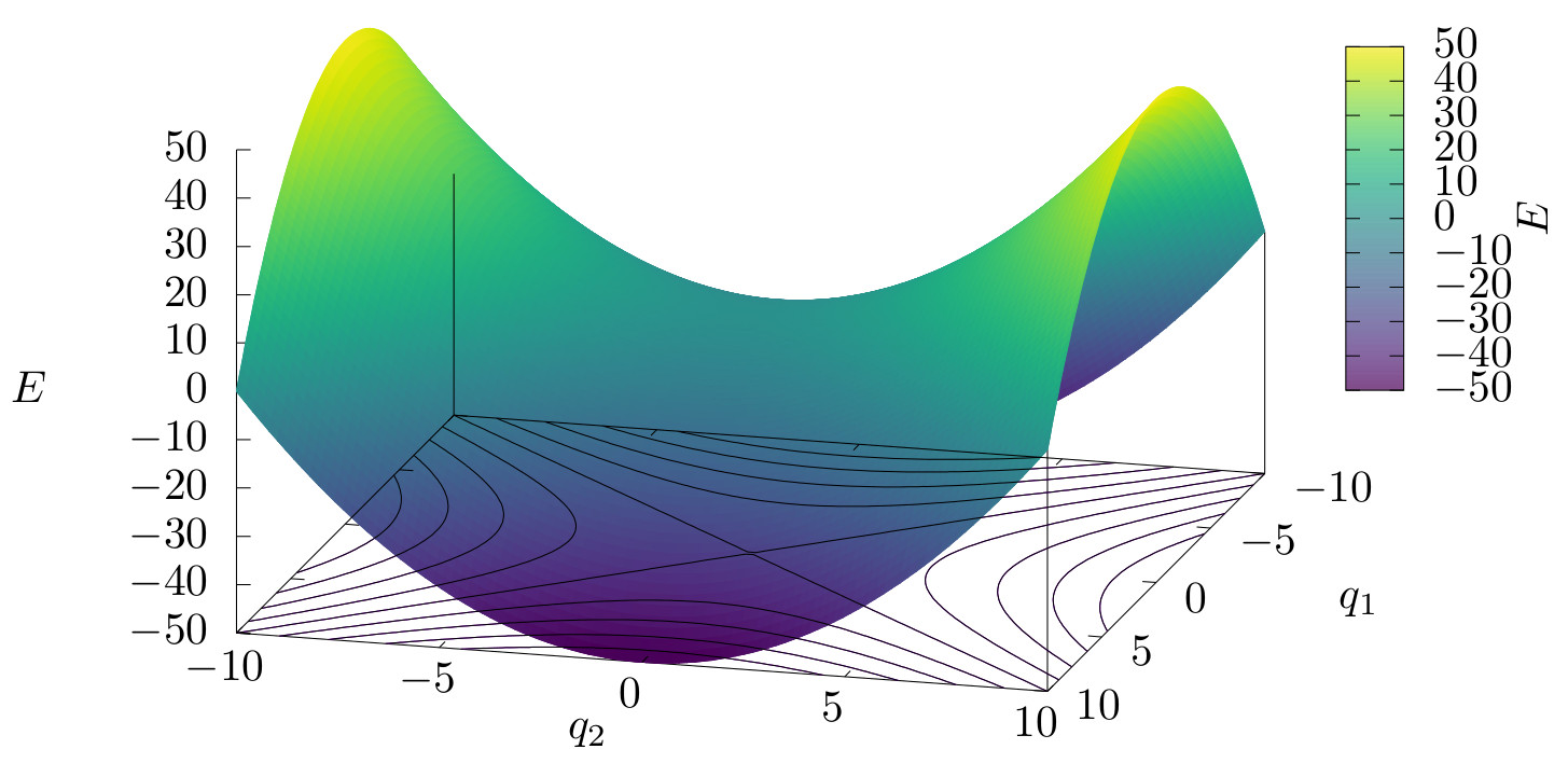
(27)¶\[\begin{split}\begin{eqnarray} H &=& K(p_{1},p_{2}) + V(q_{1},q_{2}) \\ &=& K_1(p_1) + V_1(q) + K_2(p_2) + V_2(q_2) \\ &=& \frac{\lambda}{2} (p^2_1 - q^2_1) + \frac{\omega}{2} (p^2_2 + q^2_2),\quad \lambda, \omega >0 \end{eqnarray}\end{split}\]

Fig. 3 Potential energy associated to the 2-degree of freedom system \(V(q_1,q_2) = V_1(q_1)+V_2(q_2)\). The potential has a saddle point at the point \((q_1, q_2)=(0,0)\)¶

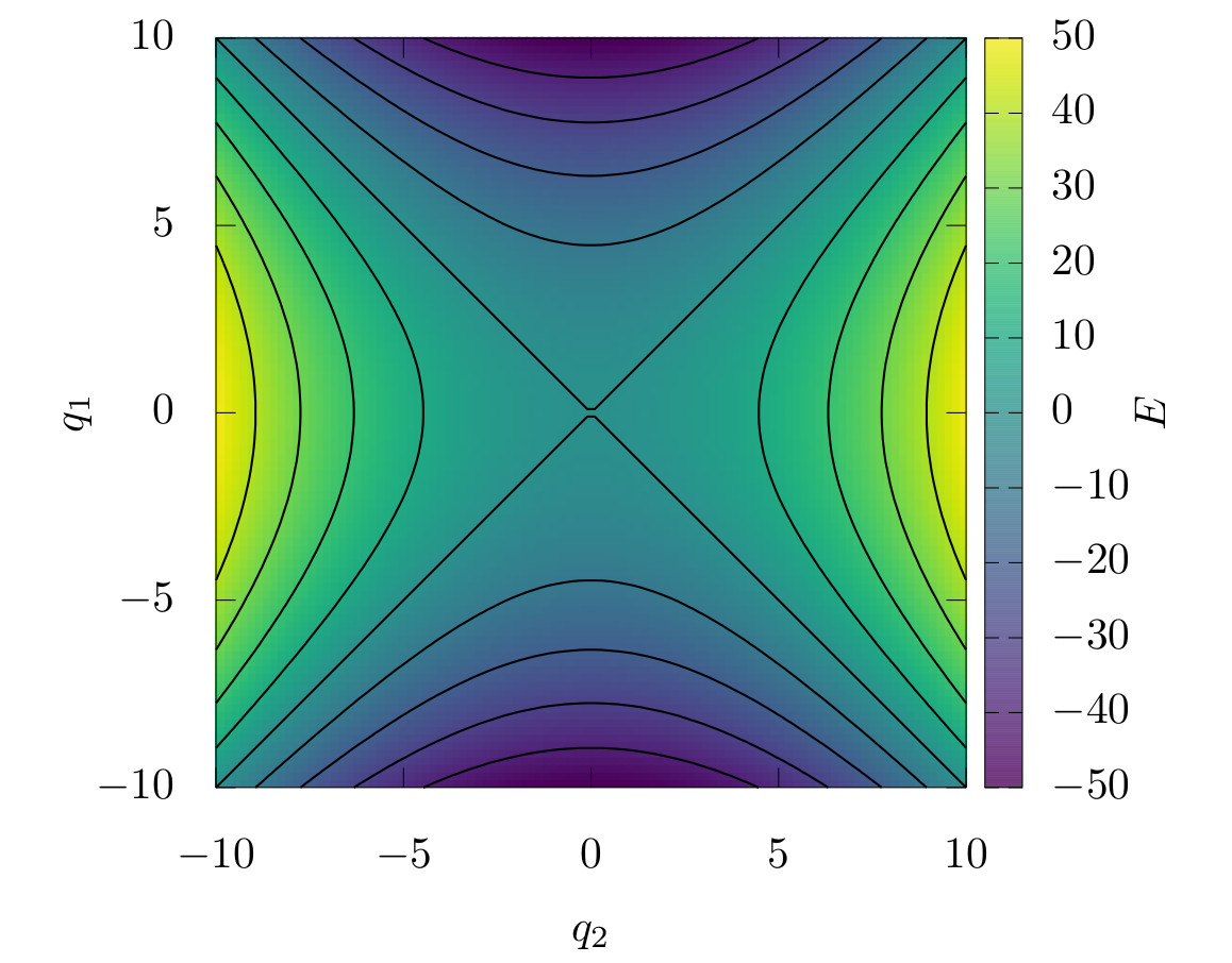
Fig. 4 Contour plot of \(V(q_1,q_2)\). The black curves are the equipotential curves.¶

Hamilton’s equations are

(28)¶\[\begin{split}\begin{eqnarray} \dot{q_1} &=& \frac{\partial H}{ \partial p_1} = \lambda p_1 \\ \dot{p_1} &=& -\frac{\partial H}{ \partial q_1} = \lambda q_1 \\ \dot{q_2} &=& \frac{\partial H}{ \partial p_2} = \omega p_2 \\ \dot{p_2} &=& -\frac{\partial H}{ \partial q_2} = -\omega q_2 \end{eqnarray}\end{split}\]

Fig. 5 (a) Potential \(V_1(q_1)\)¶

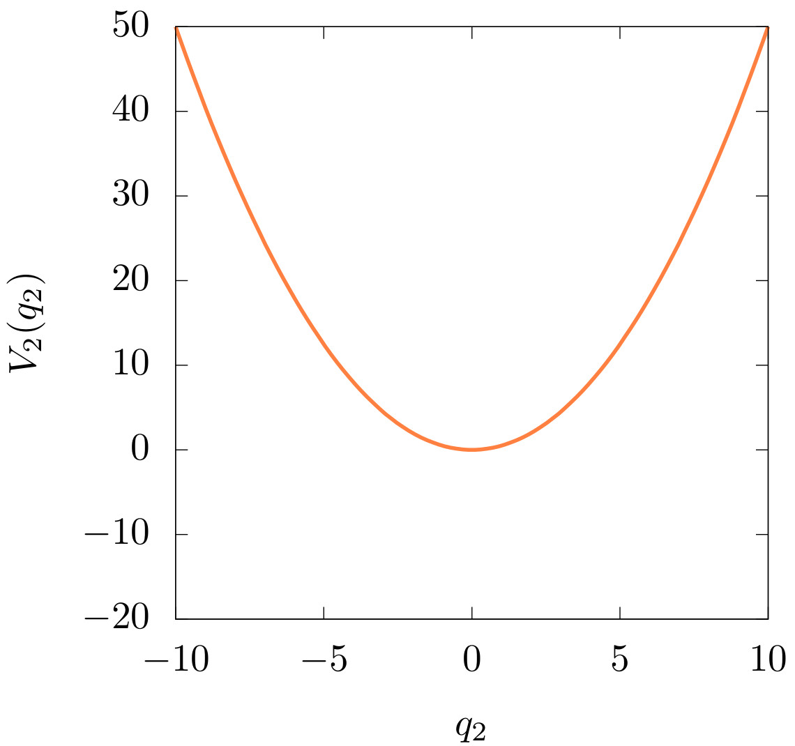
Fig. 6 (b) Potential \(V_2(q_2)\)¶

Fig. 7 (c) Plane \(q_1\)–\(p_1\)¶

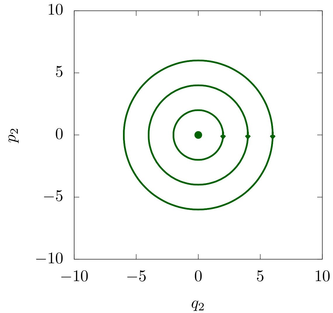
Fig. 8 (d) Plane \(q_2\)–\(p_2\)¶

Again, the point in the phase space \((q_1,q_2,p_1,p_2)=(0,0,0,0)\) is a equilibrium point of the system at the energy \(E=0\). The equilibrium point has stable and unstable manifolds, similar to the 1-degree of freedom example above.

For any \(E_2>0\) and \(E_1=0\), i.e \(E=E_2\), a periodic orbit \(\gamma\) exists in the \((q_2,p_2)\) plane and this periodic orbit is unstable.

(29)¶\[\begin{equation} \displaystyle{\gamma = \lbrace (0,q_2, 0,p_2 ) | \frac{\omega}{2} (p^2_2 + q^2_2) = E > 0 \rbrace}. \label{eq:NHIM} \end{equation}\]

In a similar way to the 1-degree of freedom case, we can find the stable and unstable manifolds of the periodic orbit \(\gamma\). To find \(W^u(\gamma)\) and \(W^s(\gamma)\) in this two degree of freedom system, it is necessary to consider the composition of the oscillation in \(q_2\) direction and the motion along the stable and unstable manifolds associated to the 1-degree of freedom case studied before. The stable and unstable manifolds of \(\gamma\) are

(30)¶\[\begin{equation} \displaystyle{ W^u(\gamma)= \lbrace (q_1,q_2, p_1,p_2 ) | \frac{\omega}{2} (p^2_2 + q^2_2) = E > 0, q_1 = p_1 \rbrace }. \end{equation}\]

(31)¶\[\begin{equation} \displaystyle{ W^s(\gamma)= \lbrace (q_1,q_2, p_1,p_2 ) | \frac{\omega}{2} (p^2_2 + q^2_2) = E > 0, q_1 = - p_1 \rbrace }. \end{equation}\]

Three and More Degrees-of-Freedom and NHIMs¶

Let us consider the most simple example with \(n\) degrees of freedom. The basic idea is the same as in the previous example with 2 degrees of freedom, where the dynamics of each degree of freedom is independent from the other degrees of freedom. In this case, the most simple Hamiltonian function of a \(n\) degree of freedom is

(32)¶\[\begin{equation} H = \frac{\lambda}{2} (p^2_1 - q^2_1)+ \sum^n_{i=2} \frac{\omega_i}{2} (p^2_i + q^2_i), \end{equation}\]

where \(\lambda, \omega_i >0\).

The equation of motion are :

(33)¶\[\begin{split}\begin{eqnarray} \dot{q_1} &=& \frac{\partial H}{ \partial p_1} = \lambda p_1\\ \dot{p_1} &=& -\frac{\partial H}{ \partial q_1} = \lambda q_1\\ \dot{q_i} &=& \frac{\partial H}{ \partial p_i} = \omega_i p_i\\ \dot{p_i} &=& -\frac{\partial H}{ \partial q_i} = -\omega_i q_i, \quad i = 2,...,n. \end{eqnarray}\end{split}\]

Fig. 9 (a) Potential \(V_1(q_1)\)¶

Fig. 10 (b) Potential \(V_2(q_2)\)¶

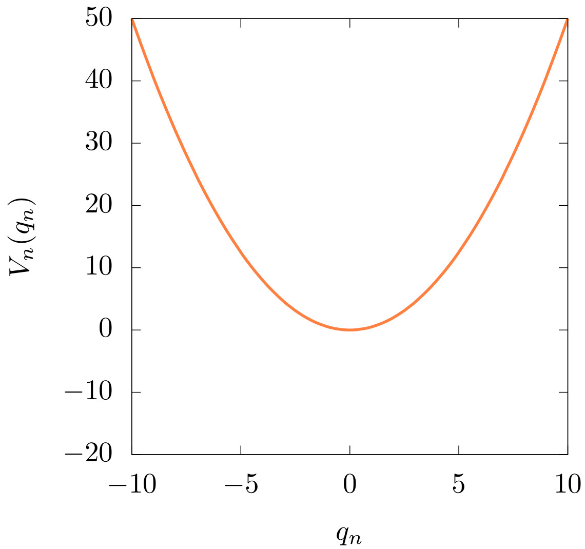
Fig. 11 (c) Potential \(V_n(q_n)\)¶

Fig. 12 (d) Plane \(q_1\)–\(p_1\)¶

Fig. 13 (e) Plane \(q_2\)–\(p_2\)¶

Fig. 14 (f) Plane \(q_n\)–\(p_n\).¶

The NHIM and its stable and unstable manifolds can be found analogously to the 2 degree of freedom system case. If \(q_1=p_1=0\) then \(\dot{q_1}=0\) and \(\dot{p_1}=0\) and the system consists of \(n-1\) harmonic oscillators bounded by the fixed total energy. For \(E=0\), \(q_1,p_1=0\) is an unstable equilibrium point and for \(E>0\), an invariant set that can be shown to be a sphere. The dimension of the sphere depends on the number of degrees of freedom with non-zero energy. This sphere is a manifold, it is invariant and normally hyperbolic, hence a NHIM. In general a NHIM does not have to be a sphere. If all degrees of freedom have non-zero energy, except for \(q_1,p_1=0\), the NHIM is \(2n-3\) dimensional and its stable and unstable manifolds are dynamical barriers on the energy level set according to Table 1 .

(34)¶\[\begin{equation} \displaystyle{ \Gamma = \lbrace (0,q_2,...,q_n, 0,p_2,...,p_n ) | \sum_{i=2}^n \frac{\omega_i}{2} (p^2_i + q^2_i) = E > 0,\rbrace } \end{equation}\]

Note that the NHIM is a generalization of the hyperbolic equilibrium point and hyperbolic periodic orbit from previous examples.

The stable and unstable manifolds, \(W^{u}(\Gamma)\) and \(W^{s}(\Gamma)\), are multidimensional cylinders that intersect in the multidimensional sphere \(\Gamma\).

(35)¶\[\begin{equation} \displaystyle{ W^u(\Gamma)= \lbrace (q_1,q_2,...,q_n, p_1,p_2,...,p_n ) | \sum^n_{i=2} \frac{\omega_i}{2} (p^2_i + q^2_i) = E > 0, q_1 = p_1 \rbrace }. \end{equation}\]

(36)¶\[\begin{equation} \displaystyle{ W^s(\Gamma)= \lbrace (q_1,q_2,...,q_n, p_1,p_2,...,p_n ) | \sum^n_{i=2} \frac{\omega_i}{2} (p^2_i + q^2_i) = E > 0, q_1 = - p_1 \rbrace }. \end{equation}\]

The general study of NHIMs, including their characterization, the nature of their invariant manifolds, and their properties under perturbations for more general systems are discussed in the works by Fenichel [Fen71][Fen74][Fen77] and more recent works [Wig94][Eld13].

It is important to note that the basic theory of NHIMs does not tell us how to find NHIMs in specific systems. It only characterizes them and describes their properties based on that characterization. Next we describe a theorem from Hamiltonian systems that provides sufficient conditions for the existence of NHIMs under certain specific circumstances.

The Lyapunov Subcenter Theorem¶

The Lyapunov subcenter theorem [Lia07] is a fundamental theorem in Hamiltonian mechanics that describes how index one saddle points of Hamilton’s equations give rise to periodic orbits, or ``NHIMs’’. Basic background on the topic can be found in [Mos58][Kel67][Mos76][Wei73][Dui72].

We will explain the ideas in the context of a two degree-of-freedom quadratic Hamiltonian, and then describe how they extend to more general settings.

(37)¶\[\begin{equation} H = \frac{\lambda}{2} (p_1^2 - q_1^2) + \frac{\omega}{2} ( p_2^2 + q_2^2), \quad \lambda, \, \omega >0, \quad (q_1, p_1, q_2, p_2) \in \mathbb{R}^4, \label{eq:LST1} \end{equation}\]

with corresponding Hamilton’s equations:

(38)¶\[\begin{split}\begin{eqnarray} \dot{q}_1 & = & \frac{\partial H}{\partial p_1} = \lambda p_1, \\ \dot{p}_1 & = & - \frac{\partial H}{\partial q_1} = \lambda q_1, \\ \dot{q}_2 & = & \frac{\partial H}{\partial p_2} = \omega p_2, \\ \dot{p}_2 & = & - \frac{\partial H}{\partial q_2} = - \omega q_2, \label{eq:LST2} \end{eqnarray}\end{split}\]

The point \((q_1, p_1, q_2, p_2) = (0, 0, 0, 0)\) is an equilibrium point of Hamilton’s equations, and the eigenvalues of the matrix associated with the linearization of Hamilton’s equations about this equilibrium point are \(\pm \lambda, \, \pm i \omega\). Hence, this equilibrium point is an index one saddle point. Note that the total energy of this equilibrium point, i.e. the value of the Hamiltonian (37) evaluated at the equilibrium point, is zero.

(39)¶\[\begin{equation} \frac{\lambda}{2} (p_1^2 - q_1^2) + \frac{\omega}{2} ( p_2^2 + q_2^2)=E >0, \label{eq:LST3} \end{equation}\]

We now want to show that for energies above the index one saddle, i.e. \(E>0\), there is a two dimensional invariant manifold of unstable periodic orbits.

First, note that \(q_1 = p_1 =0\) is an invariant manifold for all values of \(E\). We can compute the intersection of this invariant manifold by substituting \(q_1 = p_1 =0\) into the energy equation to obtain:

(40)¶\[\begin{equation} \frac{\omega}{2} ( p_2^2 + q_2^2)=E >0, \label{eq:LST4} \end{equation}\]

which is a periodic orbit for each \(E > 0\). It is instructive to count the dimensions for intersecting sets. The phase space is four dimensional, the energy surface is three dimensional, and \(q_1 = p_1 =0\) is two dimensional. A three dimensional surface intersects a two dimensional surface in a four dimensional space in a one dimensional set, which is the periodic orbit (40) . This family of periodic orbits (“family” in terms of the energy \(E>0\), lies on the two dimensional invariant manifold \(q_1 = p_1 =0\). This is the Lyapunov subcenter manifold. Note that the Lyapunov subcenter manifold is not isoenergetic. Each periodic orbit has a different energy, monotonically increasing from zero, which is the energy of the index one saddle point.

The Lyapunov subcenter theorem says that this result holds, for sufficiently small \(E > 0\), if higher order terms are added to (37) . All of these periodic orbits are unstable since the dynamics normal to the Lyapunov subcenter manifold is exponentially growing and decaying, i.e. the Lyapunov subcenter manifold is a NHIM.

This set-up can be generalized to higher dimensions. The quadratic normal form associated to an index \(n_s\) saddle has the general form (assuming that the \(\lambda_i\) are distinct and the \(\omega_i\) are distinct):

(41)¶\[\begin{equation} H =\sum_{i=1}^{n_s} \frac{\lambda_i}{2} (p_i^2 - q_i^2) + \sum_{i=1}^{n_c}\frac{\omega_{i+n_s}}{2} ( p_{i+n_s}^2 + q_{i+n_s}^2), \label{eq:LST5} \end{equation}\]

where \(\lambda_i, \, \omega_i >0, \quad (q_1, p_1, \ldots, q_{n_s}, p_{n_s}, q_{n_s +1}, p_{n_s + 1}, \ldots, q_{n_s +n_c}, p_{n_s + n_c}) \in \mathbb{R}^{2(n_s + n_c)}\).

The structure of the NHIM is treated in detail for \({n_s} =1\) in [Wig16a]. Results for \({n_s} >1\) are treated in [CEW11].

Lagrangian Descriptors

The Hyperbolic setting¶

One Degree-of-Freedom Hyperbolic Equilibrium Point¶

Two Degrees-of-Freedom and the Hyperbolic Periodic Orbit¶

Three and More Degrees-of-Freedom and NHIMs¶

The Lyapunov Subcenter Theorem¶

References¶

References

- Arnold13
V. I. Arnol’d. Mathematical methods of classical mechanics. Volume 60. Springer Science & Business Media, 2013.
- Arn62
V. I. Arnold. The classical theory of perturbations and the problem of stability of planetary systems. Soviet Mathematics Doklady, 3:1008–1012, 1962.
- Arn63a
V. I. Arnold. Proof of a theorem of A. N. Kolmogorov on the invariance of quasi-periodic motions under small perturbations of the Hamiltonian. Russian Mathematical Surveys, 18(5):9–36, 1963.
- Arn63b
V. I. Arnold. Small divisor problems in classical and celestial mechanics. Russian Mathematical Surveys, 18(6):85–192, 1963.
- BG97
J. Barrow-Green. Poincaré and the three body problem. Number 11. American Mathematical Soc., 1997.
- Chi79
B. V. Chirikov. A universal instability of many-dimensional oscillator systems. Physics Reports, 52(5):263–379, 1979. doi:https://doi.org/10.1016/0370-1573(79)90023-1.
- CEW11
P. Collins, G. S Ezra, and S. Wiggins. Index k saddles and dividing surfaces in phase space with applications to isomerization dynamics. The Journal of chemical physics, 134(24):244105, 2011.
- DH96
F. Diacu and P. Holmes. Celestial Encounters: The Origins of Chaos and Stability. Princeton University Press, 1996.
- Dui72
JJ Duistermaat. On periodic solutions near equilibrium points of conservative systems. Archive for Rational Mechanics and Analysis, 45(2):143–160, 1972.
- Dum14
H. S. Dumas. The KAM Story: A Friendly Introduction to the Content, History, and Significance of Classical Kolmogorovâ Arnoldâ Moser Theory. World Scientific Publishing Company, 2014.
- Eld13(1,2)
J Eldering. Normally Hyperbolic Invariant Manifolds. The Noncompact Case. Atlantis Press, 2013.
- Fen71(1,2)
N Fenichel. Persistence and smoothess of the invariant manifolds for flows. Indiana University Mathematics Journal, 1971.
- Fen74
N. Fenichel. Asymptotic stability with rate conditions. Indiana Univ. Math. J., 23:1109–1137, 1974.
- Fen77
N. Fenichel. Asymptotic stability with rate conditions, ii. Indiana Univ. Math. J., 26:81–93, 1977.
- Gio02
A. Giorgilli. Notes on Exponential stability of Hamiltonian systems. Centro de ricerca Matematica Ennio De Giorgi Pisa, February 4-15., 2002.
- GP10
Victor Guillemin and Alan Pollack. Differential topology. Volume 370. American Mathematical Soc., 2010.
- Kel67
A. Kelley. On the liapounov subcenter manifold. Journal of mathematical analysis and applications, 18(3):472–478, 1967.
- Kol57
A. N. Kolmogorov. Théorie générale des systèmes dynamiques et mécanique classique. In Proceedings of the International Congress of Mathematicians, Amsterdam, 1954, Vol. 1, 315–333. North-Holland Publishing Co., 1957.
- Lia07
A. Liapounoff. Problème général de la stabilité du mouvement. In Annales de la Faculté des sciences de Toulouse: Mathématiques, volume 9, 203–474. 1907.
- Lio55
J. Liouville. Note sur l’intégration des équations différentielles de la dynamique, présentée au bureau des longitudes le 29 juin 1853. Journal de Mathématiques pures et appliquées, pages 137–138, 1855.
- MM74
Lawrence Markus and Kenneth Ray Meyer. Generic Hamiltonian dynamical systems are neither integrable nor ergodic. Number 144. American Mathematical Soc., 1974.
- Mei08
J. D. Meiss. Visual explorations of dynamics: The standard map. Pramana, 70(6):965–988, 2008. doi:10.1007/s12043-008-0103-3.
- Min35
H. Mineur. Sur les systemes mécaniques admettant n intégrales premieres uniformes et l’extensiona ces systemes de la méthode de quantification de sommerfeld. CR Acad. Sci., Paris, 200:1571–1573, 1935.
- Min37
H. Mineur. Sur les systèmes mécaniques dans lesquels figurent des paramètres fonctions du temps. Étude des systèmes admettant n intégrales premières uniformes en involution. extension à ces systèmes des conditions de quantification de bohr-sommerfeld. J. Ecole Polytechn, 3:173–191, 1937.
- Mos58
J. Moser. On the generalization of a theorem of a. liapounoff. Communications on Pure and Applied Mathematics, 11(2):257–271, 1958.
- Mos76
J. Moser. Periodic orbits near an equilibrium and a theorem by alan weinstein. Communications on Pure and Applied Mathematics, 29(6):727–747, 1976.
- Mos01
J. Moser. Stable and random motions in dynamical systems: With special emphasis on celestial mechanics. Volume 1. Princeton university press, 2001.
- Mos62
J. K. Moser. On invariant curves of area-preserving mappings of an annulus. Nachr. Akad. Wiss. Göttingen II, Math. Phys. Kl., pages 1–20, 1962.
- Wei73
A. Weinstein. Normal modes for nonlinear hamiltonian systems. Inventiones mathematicae, 20(1):47–57, 1973.
- Wig90
S Wiggins. On the geometry of transport in phase space I. transport in k-degree-of-freedom hamiltonian systems, $2 \le k< \infty $. Physica D: Nonlinear Phenomena, 44(3):471–501, 1990.
- Wig94(1,2)
S Wiggins. Normally hyperbolic invariant manifolds in dynamical systems. Springer-Verlag New York, 1994.
- Wig04
S Wiggins. Introduction to Applied Nonlinear Dynamics and Chaos. Springer–Verlag, 2004.
- WWJaffeU01(1,2)
S Wiggins, L Wiesenfeld, C Jaffé, and T Uzer. Impenetrable Barriers in Phase-Space. Phys. Rev. Lett., 86(24):5478–5481, jun 2001. URL: https://link.aps.org/doi/10.1103/PhysRevLett.86.5478, doi:10.1103/PhysRevLett.86.5478.
- Wig03
S. Wiggins. Introduction to applied nonlinear dynamical systems and chaos. Volume 2. Springer Science & Business Media, 2003.
- Wig16a
S. Wiggins. The role of normally hyperbolic invariant manifolds (nhims) in the context of the phase space setting for chemical reaction dynamics. Regular and Chaotic Dynamics, 21(6):621–638, 2016.
- Wig16b
S. Wiggins. The role of normally hyperbolic invariant manifolds (NHIMS) in the context of the phase space setting for chemical reaction dynamics. Regular and Chaotic Dynamics, 21(6):621–638, 2016.