The Method of Lagrangian Descriptors¶

Introduction¶

One of the biggest challenges of dynamical systems theory or nonlinear dynamics is the development of mathematical techniques that provide us with the capability of exploring transport in phase space. Since the early 1900, the idea of pursuing a qualitative description of the solutions of differential equations, which emerged from the pioneering work carried out by Henri Poincaré on the three body problem of celestial mechanics [Poincare90], has had a profound impact on our understanding of the nonlinear character of natural phenomena. The qualitative theory of dynamical systems has now been widely embraced by the scientific community.

The goal of this section is to describe the details behind the method of Lagrangian descriptors. This simple and powerful technique unveils regions with qualitatively distinct dynamical behavior, the boundaries of which consist of invariant manifolds. In a procedure that is best characterised as phase space tomography, we can use low-dimensional slices we are able to completely reconstruct the intricate geometry of underlying invariant manifolds that governs phase space transport.

Consider a general time-dependent dynamical system given by the equation:

(48)¶\[\begin{equation} \dfrac{d\mathbf{x}}{dt} = \mathbf{f}(\mathbf{x},t) \;,\quad \mathbf{x} \in \mathbb{R}^{n} \;,\; t \in \mathbb{R} \;, \label{eq:gtp_dynSys} \end{equation}\]

where the vector field $\mathbf{f}(\mathbf{x},t)$ is assumed to be sufficiently smooth both in space and time. The vector field $\mathbf{f}$ can be prescribed by an analytical model or given from numerical simulations as a discrete spatio-temporal data set. For instance, the vector field could represent the velocity field of oceanic or atmospheric currents obtained from satellite measurements or from the numerical solution of geophysical models. In the context of chemical reaction dynamics, the vector field could be the result of molecular dynamics simulations. For any initial condition $\mathbf{x}(t_0) = \mathbf{x}_0$, the system of first order nonlinear differential equations given in Eq. (48) has a unique solution represented by the trajectory that starts from that initial point $\mathbf{x}_0$ at time $t_0$.

Since all the information that determines the behavior and fate of the trajectories for the dynamical system is encoded in the initial conditions (ICs) from which they are generated, we are interested in the development of a mathematical technique with the capability of revealing the underlying geometrical structures that govern the transport in phase space.

Lagrangian descriptors (LDs) provide us with a simple and effective way of addressing this challenging task, because it is formulated as a scalar trajectory-diagnostic tool based on trajectories. The elegant idea behind this methodology is that it assigns to each initial condition selected in the phase space a positive number, which is calculated by accumulating the values taken by a predefined positive function along the trajectory when the system is evolved forward and backward for some time interval. The positive function of the phase space variables that is used to define different types of LD might have some geometrical or physical relevance, but this is not a necessary requirement for the implementation of the method. This approach is remarkably similar to the visualization techniques used in laboratory experiments to uncover the beautiful patterns of fluid flow structures with the help of drops of dye injected into the moving fluid [CRO86]. In fact, the development of LDs was originally inspired by the desire to explain the intricate geometrical flow patterns that are responsible for governing transport and mixing processes in Geophysical flows. The method was first introduced a decade ago based on the arclength of fluid parcel trajectories [MM09][MM10]. Regions displaying qualitatively distinct dynamics will frequently contain trajectories with distinct arclengths and a large variation of the arclength indicate the presence of separatrices consisting of invariant manifolds [MWCM13].

Lagrangian descriptors have advantages in comparison with other methodologies for the exploration of phase space structures. A notable advantage is that they are straightforward to implement. Since its proposal as a nonlinear dynamics tool to explore phase space, this technique has found a myriad of applications in different scientific areas. For instance, it has been used in oceanography to plan transoceanic autonomous underwater vehicle missions by taking advantage of the underlying dynamical structure of ocean currents [RGarciaGM+18]. Also, it has been shown to provide relevant information for the effective management of marine oil spills [GGRM+16]. LDs have been used to analyze the structure of the Stratospheric Polar Vortex and its relation to sudden stratospheric warmings and also to ozone hole formation [dlCamaraMI+12][dlCamaraMM+13][CMMW19a][CMMW19b]. In all these problems, the vector field defining the dynamical system is a discrete spatio-temporal dataset obtained from the numerical simulation of geophysical models. Recently, this tool has also received recognition in the field of chemistry, for instance in transition state theory [CH15][CH16][CJH17][RBB19], where the computation of chemical reaction rates relies on the know-ledge of the phase space structures. These high-dimensional structures characterizing reaction dynamics are typically related to Normally Hyperbolic Invariant Manifolds (NHIMs) and their stable and unstable manifolds that occur in Hamiltonian systems. Other applications of LDs to chemical problems include the analysis of isomerization reactions [NW20][GarciaGAW20], roaming [KrajvnakEW19][MW20a], the study of the influence of bifurcations on the manifolds that control chemical reactions [GarciaGNW20], and also the explanation of the dynamical matching mechanism in terms of the existence of heteroclinic connections in a Hamiltonian system defined by Caldera-type potential energy surfaces [KGarciaGW20].

Lagrangian Descriptors versus Poincaré Maps¶

Poincaré maps have been a standard and traditional technique for understanding the global phase space structure of dynamical systems. However, Lagrangian descriptors offer substantial advantages over Poincaré maps. We will describe these advantages in the context of the most common settings in which they are applied. However, we note that Lagrangian descriptors can be applied in exactly the same way to both Hamiltonian and non-Hamiltonian vector fields. In keeping with the spirit of this book, we will frame our discussion and description in the Hamiltonian setting.

Autonomous Hamiltonian vector fields¶

The consideration of the dimension of different geometric objects is crucial to understanding the advantages of Lagrangian descriptors over Poincaré maps. Therefore we will first consider the “simplest” situation in which these arise — the autonomous Hamiltonian systems with two degrees of freedom.

A two degree-of-freedom Hamiltonian system is described by a four dimensional phase space described by coordinates $(q_1, q_2, p_1, p_2)$. Moreover, we have seen in Section REF that trajectories are restricted to a three dimensional energy surface (“energy conservation in autonomous Hamiltonian systems”). We choose a two dimensional surface within the energy surface that is transverse to the Hamiltonian vector field. This means that at no point on the two dimensional surface is the Hamiltonian vector field tangent to the surface and that at every point on the surface the Hamiltonian vector field has the same directional sense (this is defined more precisely in REF). This two dimensional surface is referred to as a surface of section (SOS) or a Poincaré section, and it is the domain of the Poincaré map. The image of a point under the Poincaré map is the point on the trajectory, starting from that point, that first returns to the surface (and this leads to the fact that the Poincaré map is sometimes referred to as a “first return map”).

The practical implementation of this procedure gives rise to several questions. Given a specific two degree-of-freedom Hamiltonian system can we find a two dimensional surface in the three dimensional energy surface having the property that it is transverse to the Hamiltonian vector field and “most” trajectories with initial conditions on the surface return to the surface? In general, the answer is “no” (unless we have some useful a priori knowledge of the phase space structure of the system). The advantage of the method of Lagrangian descriptors is that none of these features are required for its implementation, and it gives essentially the same information as Poincaré maps.

However, the real advantage comes in considering higher dimensions, e.g autonomous Hamiltonian systems with more than two degrees-of-freedom. For definiteness, we will consider a three degree-of-freedom autonomous Hamiltonian system. In this case the phase space is six dimensional and the energy surface is five dimensional. A cross section to the energy surface, in the sense described above, would be four dimensional (if an appropriate cross-section could be found). Solely on dimensionality considerations, we can see the difficulty. Choosing “enough” initial conditions on this four dimensional surface so that we can determine the phase space structures that are mapped out by the points that return to the cross-section is “non-trivial” (to say the least), and the situation only gets more difficult when we go to more than three degrees-of-freedom. One might imagine that you could start by considering lower dimensional subsets of the cross section. However, the probability that a trajectory would return to a lower dimensional subset is zero. Examples where Lagrangian descriptors have been used to analyse phase space structures in two and three degree-of-freedom Hamiltonian systems with this approach are given in [DW17][NGarciaGW19][NW19][GarciaGNW19].

Lagrangian descriptors avoid all of these difficulties. In particular, they can be computed on any subset of the phase space since there is no requirement for trajectories to return to that subset. Since phase space structure is encoded in the initial conditions (not the final state) of trajectories a dense grid of initial conditions can be placed on any subset of the phase space and a “Lagrangian descriptor field” can be computed for that subset with high resolution and accuracy. Such computations are generally not possible using the Poincaré map approach.

Nonautonomous Hamiltonian vector fields¶

Nonautonomous vector fields are fundamentally different than autonomous vector fields, and even more so for Hamiltonian vector fields. For example, one degree-of-freedom autonomous Hamiltonian vector fields are integrable. One degree-of-freedom autonomous Hamiltonian vector fields may exhibit chaos. Regardless of the dimension, a very significant difference is that energy is not conserved for nonautonomous Hamiltonian vector fields. Nevertheless, Lagrangian descriptors can be applied in exactly the same way as for autonomous Hamiltonian vector fields, regardless of the nature of the time dependence. We add this last remark since the concept of Poincaré maps is not applicable unless the time dependence is periodic.

Formulations for Lagrangian Descriptors¶

The Arclength Definition¶

In order to build some intuition on how the method works and understand its very simple and straightforward implementation, we start with the arclength definition mentioned in the previous section. This version of LDs is also known in the literature as function $M$. Consider any region of the phase space where one would like to reveal structures at time $t = t_0$, and create a uniformly-spaced grid of ICs $\mathbf{x}_0 = \mathbf{x}(t_0)$ on it. Select a fixed integration time $\tau$ that will be used to evolve all the trajectories generated from these ICs forward and backward in time for the time intervals $[t_0,t_0+\tau]$ and $[t_0-\tau,t_0]$ respectively. This covers a temporal range of $2\tau$ centered at $t = t_0$, marking the time at which we want to take a snapshot of the underlying structures in phase space. The arclength of a trajectory in forward time can be easily calculated by solving he integral:

(49)¶\[\begin{equation} \mathcal{L}^{f}(\mathbf{x}_{0},t_0,\tau) = \int^{t_0+\tau}_{t_0} ||\dot{\mathbf{x}}|| \; dt \;, \label{eq:M_function_fw} \end{equation}\]

where $\dot{\mathbf{x}} = \mathbf{f}(\mathbf{x}(t;\mathbf{x}_0),t)$ and $||\cdot||$ is the Euclidean norm applied to the vector field defining the dynamical system in Eq. (48) . Similarly, one can define the arclength when the trajectory evolves in backward time as:

(50)¶\[\begin{equation} \mathcal{L}^{b}(\mathbf{x}_{0},t_0,\tau) = \int^{t_0}_{t_0-\tau} ||\dot{\mathbf{x}}|| \; dt \;, \label{eq:M_function_bw} \end{equation}\]

It is common practice to combine these two quantities into one scalar value so that:

(51)¶\[\begin{equation} \mathcal{L}(\mathbf{x}_{0},t_0,\tau) = \mathcal{L}^{b}(\mathbf{x}_{0},t_0,\tau) + \mathcal{L}^{f}(\mathbf{x}_{0},t_0,\tau) \;, \label{eq:M_function} \end{equation}\]

and in this way the scalar field provided by the method will simultaneously reveal the location of the stable and unstable manifolds in the same picture. However, if one only considers the output obtained from the forward or backward contributions, we can separately depict the stable and unstable manifolds respectively.

We illustrate the logic behind the capabilities of this technique to display the stable and unstable manifolds of hyperbolic points with a very simple example, the one degree-of-freedom (DoF) linear Hamiltonian saddle system given by:

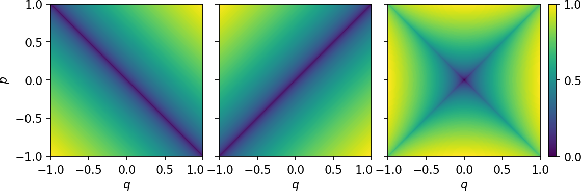
(52)¶\[\begin{split}\begin{equation} H(q,p) = \dfrac{1}{2} \left(p^2 - q^2\right) \quad \Leftrightarrow \quad \begin{cases} \dot{q} = \dfrac{\partial H}{\partial p} = p \\[.4cm] \dot{p} = -\dfrac{\partial H}{\partial q} = q \end{cases} \label{eq:1dof_saddle} \end{equation}\end{split}\]

Fig. 24 Forward (50), backward (49) and combined (51) Lagrangian descriptors for system (52) respectively.¶

We know that this dynamical system has a hyperbolic equilibrium point at the origin and that its stable and unstable invariant manifolds correspond to the lines $p = \pm q$ respectively (refer to hyperbolic section). Outside of these lines, the trajectories are hyperbolas. What happens when we apply LDs to this system? Why does the method pick up the manifolds? Notice first that in Fig. 24 the value attained by LDs at the origin is zero, because it is an equilibrium point and hence it is not moving. Therefore, the arclength of its trajectory is zero. Next, let’s consider the forward time evolution term of LDs, that is, $\mathcal{L}^f$. Take two neighboring ICs, one lying on the line that corresponds to the stable manifold and another slightly off it. If we integrate them for a time $\tau$, the initial condition that is on the manifold converges to the origin, while the other initial condition follows the arc of a hyperbola. If $\tau$ is small, both segments of trajectory are comparable in length, so that the value obtained from LDs for both ICs is almost equal. However, if we integrate the system for a larger $\tau$, the arclengths of the two trajectories become very different, because one converges while the other one diverges. Therefore, we can clearly see in Fig. 24 that the LD values vary significantly near the stable manifold in comparison to those elsewhere. Moreover, if we consider a curve of initial conditions that crosses transversely the stable manifold, the LD value along it attains a minimum on the manifold. Notice also that by the same argument we gave above, but constructing the backward time evolution term of LDs, $\mathcal{L}^b$, we can arrive to the conclusion that backward integration of initial conditions will highlight the unstable manifold of the hyperbolic equilibrium point at the origin. It is important to remark here that, although we have used above the simple linear saddle system as an example to illustrate how the method recovers phase space structure, this argument also applies to a nonlinear system with an hyperbolic point, whose stable and unstable manifolds are convoluted curves.

The sharp transitions obtained for the LD values across the stable and unstable manifolds, which imply large values of its gradient in the vicinity of them, are known in the literature as “singular features”. These features present in the LD scalar field are very easy to visualize and detect when plotting the output provided by the method. We will see shortly that there exists a rigorous mathematical connection between the “singular features” displayed by the LD output and the stable and unstable manifolds of hyperbolic points. This result was first proved in [LBIGarciaG+17] for two-dimensional flows, it was extended to 3D dynamical systems in [GarciaGCM+18], and it has also been recently established for the stable and unstable manifolds of normally hyperbolic invariant manifolds in Hamiltonian systems with two or more degrees of freedom in [DW17][NGarciaGW19]. In fact, the derivation of this relationship relies on an alternative definition for LDs, where the positive scalar function accumulated along the trajectories of the system is the $p$-norm of the vector field that determines the flow. Considering this approach, the LD scalar field becomes now non-differentiable at the phase space points that belong to a stable or unstable manifold, and consequently the gradient at these locations is unbounded. This property is crucial in many ways, since it allows us to easily recover the location of the stable and unstable manifolds in the LD plot as if they were the edges of objects that appear in a digital photograph.

One key aspect that needs to be accounted for when setting up LDs for revealing the invariant manifolds in phase space, is the crucial role that the integration time $\tau$ plays in the definition of the method itself. It is very important to appreciate this point, since $\tau$ is the parameter responsible for controlling the complexity and intricate geometry of the phase space structures revealed in the scalar field displayed from the LD computation. A natural consequence of increasing the value for $\tau$ is that richer details of the underlying structures are unveiled, since this implies that we are incorporating more information about the past and future dynamical history of trajectories in the computation of LDs. This means that $\tau$ in some sense is intimately related to the time scales of the dynamical phenomena that occur in the model under consideration. This connection makes the integration time a problem-dependent parameter, and hence, there is no general “golden rule” for selecting its value for exploring phase space. Consequently, it is usually selected from the dynamical information obtained by performing beforehand several numerical experiments, and one needs to bear in mind the compromise that exists between the complexity of the structures revealed by the method to explain a certain dynamical mechanism, and the interpretation of the intricate manifolds displayed in the LD scalar output.

To finish this part on the arclength definition of LDs we show that the method is also capable of revealing other invariant sets in phase space such as KAM tori, by means of studying the convergence of the time averages of LDs. We illustrate this property with the 1 DoF linear Hamiltonian with a center equilibrium at the origin:

(53)¶\[\begin{split}\begin{equation} H(q,p) = \dfrac{\omega}{2} \left(p^2 + q^2\right) \quad \Leftrightarrow \quad \begin{cases} \dot{q} = \dfrac{\partial H}{\partial p} = \omega \, p \\[.4cm] \dot{p} = -\dfrac{\partial H}{\partial q} = -\omega \, q \end{cases} \end{equation}\end{split}\]

From the definition of the Hamiltonian we can see that the solutions to this system form a family of concentric circles about the origin with radius $R = \sqrt{2H/\omega}$. Moreover, each of this circles encloses an area of $A(H) = 2\pi H / \omega$. Using the definition of the Hamiltonian and the information provided by Hamilton’s equations of motion we can easily evaluate the arclength LD for this system:

(54)¶\[\begin{equation} \mathcal{L}(q_0,p_0,\tau) = \int^{\tau}_{-\tau} \sqrt{\left(\dot{q}\right)^2 + \left(\dot{p}\right)^2} \; dt = \omega \int^{\tau}_{-\tau} \sqrt{q^2 + p^2} \; dt = 2 \tau \sqrt{2 \omega H_0} \end{equation}\]

where the initial condition $(q_0,p_0)$ has energy $H = H_0$ and therefore it lies on a circular trajectory with radius $\sqrt{2H_0/\omega}$. Hence, in this case all trajectories constructed from initial conditions on that circle share the same LD value. Moreover, if we consider the convergence of the time average of LD, this yields:

(55)¶\[\begin{equation} \lim_{\tau \to \infty} \langle \, \mathcal{L}(\tau) \, \rangle = \dfrac{1}{2\tau} \int^{\tau}_{-\tau} \sqrt{\left(\dot{q}\right)^2 + \left(\dot{p}\right)^2} \; dt = \sqrt{2 \omega H_0} = \omega \sqrt{\frac{A}{\pi}} \end{equation}\]

The $p$-norm Definition¶

Besides the arclength definition of Lagrangian descriptors introduced in the previous subsection, there are many other versions used throughout the literature. An alternative definition of LDs, which is inspired by the $p$-norm of the vector field describing the dynamical system. We remark that we use the expression for $p\in(0,1]$, while the $p$-norm is only a norm for $p\geq 1$. For the sake of consistency with literature we retain the name $p$-norm even for $p<1$. The LD is defined as:

(56)¶\[\begin{equation} \mathcal{L}_p(\mathbf{x}_{0},t_0,\tau) = \int^{t_0+\tau}_{t_0-\tau} \, \sum_{k=1}^{n} \vert f_{k}(\mathbf{x}(t;\mathbf{x}_0),t) \vert^p \; dt \;, \quad p \in (0,1] \label{eq:Mp_function} \end{equation}\]

where $f_{k}$ is the $k$-th component of the vector field in Eq. (48) . Typically, the value used for the parameter $p$ in this version of the method is $p = 1/2$. Recall that all the variants of LDs can be split into its forward and backward time integration components in order to detect the stable and unstable manifolds separately. Hence, we can write:

(57)¶\[\begin{equation} \mathcal{L}_p(\mathbf{x}_{0},t_0,\tau) = \mathcal{L}^{b}_p(\mathbf{x}_{0},t_0,\tau) + \mathcal{L}^{f}_p(\mathbf{x}_{0},t_0,\tau) \end{equation}\]

where we have that:

(58)¶\[\begin{split}\begin{equation} \begin{split} \mathcal{L}_p^{b}(\mathbf{x}_{0},t_0,\tau) & = \int^{t_0}_{t_0-\tau} \sum_{k=1}^{n} |f_{k}(\mathbf{x}(t;\mathbf{x}_0),t)|^p \; dt \\[.2cm] \mathcal{L}_p^{f}(\mathbf{x}_{0},t_0,\tau) & = \int^{t_0+\tau}_{t_0} \sum_{k=1}^{n} |f_{k}(\mathbf{x}(t;\mathbf{x}_0),t)|^p \; dt \end{split} \end{equation}\end{split}\]

Although this alternative definition of LDs does not have such an intuitive physical interpretation as that of arclength, it has been shown to provide many advantages. For example, it allows for a rigorous analysis of the notion of “singular features” and to establish the mathematical connection of this notion to stable and unstable invariant manifolds in phase space. Another important aspect of the $p$-norm of LDs is that, since in the definition all the vector field components contribute separately, one can naturally decompose the LD in a way that allows to isolate individual degrees of freedom. This was used in [DW17][NGarciaGW19] to show that the method can be used to successfully detect NHIMs and their stable and unstable manifolds in Hamiltonian systems. Using the $p-$norm definition, it has been shown that the points on the LD contour map with non-differentiability identifies the invariant manifolds’ intersections with the section on which the LD is computed, for specific systems [LBIGarciaG+17][DW17][NGarciaGW19]. In this context, where a fixed integration time is used, it has also been shown that the LD scalar field attains a minimum value at the locations of the stable and unstable manifolds, and hence:

(59)¶\[\begin{equation} \mathcal{W}^u(\mathbf{x}_{0},t_0) = \textrm{argmin } \mathcal{L}_p^{b}(\mathbf{x}_{0},t_0,\tau) \quad,\quad \mathcal{W}^s(\mathbf{x}_{0},t_0) = \textrm{argmin } \mathcal{L}_p^{f}(\mathbf{x}_{0},t_0,\tau) \;, \label{eq:min_LD_manifolds} \end{equation}\]

where $\mathcal{W}^u$ and $\mathcal{W}^s$ are, respectively, the unstable and stable manifolds calculated at time $t_0$ and $\textrm{argmin}(\cdot)$ denotes the phase space coordinates $\mathbf{x}_0$ that minimize the corresponding function. In addition, NHIMs at time $t_0$ can be calculated as the intersection of the stable and unstable manifolds:

(60)¶\[\begin{equation} \mathcal{N}(\mathbf{x}_{0},t_0) = \mathcal{W}^u(\mathbf{x}_{0},t_0) \cap \mathcal{W}^s(\mathbf{x}_{0},t_0) = \textrm{argmin } \mathcal{L}_p(\mathbf{x}_{0},t_0,\tau) \label{eq:min_NHIM_LD} \end{equation}\]

As we have pointed out, the location of the stable and unstable manifolds on the slice can be obtained by extracting them from the ridges of the gradient field, $\Vert \nabla \mathcal{L}^{f}_p \Vert$ or $\Vert \nabla \mathcal{L}^{b}_p \Vert$, respectively, since manifolds are located at points where the the forward and backward components of the function $\mathcal{L}_p$ are non-differentiable. Once the manifolds are known one can compute their intersection by means of a root search algorithm. In specific examples we have been able to extract NHIMs from the intersections. An alternative method to recover the manifolds and their associated NHIM is by minimizing the functions $\mathcal{L}^{f}_p$ and $\mathcal{L}^{b}_p$ using a search optimization algorithm. This second procedure and some interesting variations are described in [FSB+19].

We finish the description of the $p$-norm version of LDs by showing that this definition recovers the stable and unstable manifolds of hyperbolic equilibria at phase space points where the scalar field is non-differentiable. We demonstrate this statement for the 1 DoF linear Hamiltonian introduced in Eq. (56) that has a saddle equilibrium point at the origin. The general solution to this dynamical system can be written as:

(61)¶\[\begin{equation} q(t) = \dfrac{1}{2} \left(A e^{t} + B e^{-t}\right) \quad,\quad p(t) = \dfrac{1}{2} \left(A e^{t} - B e^{-t}\right) \end{equation}\]

where $\mathbf{x}_0 = (q_0,p_0)$ is the initial condition and $A = q_0 + p_0$ and $B = q_0 - p_0$. If we compute the forward plus backward contribution of the LD function, we get that for $\tau$ sufficiently large the scalar field behaves asymptotically as:

(62)¶\[\begin{equation} \mathcal{L}_{p}\left(\mathbf{x}_0,\tau\right) \sim \left(|A|^{p} + |B|^{p}\right) e^{p \tau} \label{eq:M_hyp_asymp} \end{equation}\]

Lagrangian Descriptors Based on the Classical Action¶

In this section we discuss a formulation of Lagrangian descriptors that has a direct connection to classical Hamiltonian mechanics, namely the principle of least action. The principle of least action is treated in most advanced books on classical mechanics; see, for example, [Arnold13][GPS02][LL13]. An intuitive and elementary discussion of the principle of least action is given by Richard Feynman in the following lecture https://www.feynmanlectures.caltech.edu/II_19.html,

To begin, we note that the general form of Lagrangian descriptors are as follows:

(63)¶\[\begin{equation} \mathcal{L}(\text{initial condition}) = \int_{t_0 - \tau}^{t_0 + \tau} \text{PositiveFunction} \, (\text{trajectory}) \; dt \end{equation}\]

The positivity of the integrand is often imposed via an absolute value. In our discussion below we show that this is not necessary for the action.

One Degree-of-Freedom Autonomous Hamiltonian Systems¶

We consider a Hamiltonian of the form:

(64)¶\[\begin{equation} H(q, p) = \frac{p^2}{2m} + V(q) \;, \quad (q,p) \in \mathbb{R}^2. \end{equation}\]

The integrand for the action integral is the following:

(65)¶\[\begin{equation} p \, dq \;, \end{equation}\]

Using the chain rule and the definition of momentum, the following calculations are straightforward:

(66)¶\[\begin{eqnarray} p \, dq = p \frac{dq}{dt} dt = \frac{p^2}{m} dt \;. \end{eqnarray}\]

The quantity $\frac{p^2}{m}$ is twice the kinetic energy and is known as the vis viva. It is the integrand for the integral that defines Maupertuis principle, which is very closely related to the principle of least action. We can also write $p \, dq$ slightly differently using Hamilton’s equations:

(67)¶\[\begin{equation} \dfrac{p^2}{m}= 2 (H - V(q) ), \end{equation}\]

from which it follows that:

(68)¶\[\begin{equation} p \, dq = \dfrac{p^2}{m} \, dt = 2 (H-V(q)) \, dt. \end{equation}\]

Therefore, the positive quantities that appear multiplying the $dt$ are candidates for the integrand of Lagrangian descriptors [MW20b].

We will illustrate next how the action-based LDs successfully detects the stable invariant manifold of the hyperbolic equilibrium point in system introduced in Eq. (52). We know that the solutions to this dynamical system are given by the expressions:

(69)¶\[\begin{equation} q(t) = q_0 \cosh(t) + p_0 \sinh(t) \quad,\quad p(t) = p_0 \cosh(t) + q_0 \sinh(t) \end{equation}\]

where $(q_0,p_0)$ represents any initial condition. We know from (refer to hyperbolic section) that the stable invariant manifold is given by $q = -p$. We compute the forward LD:

(70)¶\[\begin{split}\begin{equation} \begin{split} \mathcal{A}^{f}(q_0,p_0,\tau) & = \int_{0}^{\tau} p \, \dfrac{dq}{dt} \, dt = \int_{0}^{\tau} p^2 \, dt = \\[.2cm] & = \dfrac{1}{2} \left(p_0^2 - q_0^2\right) \tau + \dfrac{1}{4}\left(q_0^2 + p_0^2\right) \sinh(2\tau) + \dfrac{1}{2} q_0 \, p_0 \left(\cosh(2\tau) - 1\right) \end{split} \end{equation}\end{split}\]

It is a simple exercise to check that $\mathcal{A}^{f}$ attains a local minimum at the points:

(71)¶\[\begin{equation} q_0 = - \dfrac{\cosh(2\tau) - 1}{\sinh(2\tau) - 2 \tau} \, p_0 \end{equation}\]

$n$ Degree-of-Freedom Autonomous Hamiltonian Systems¶

The above calculations for one DoF are easily generalized to $n$ degrees-of-freedom. We begin with a Hamiltonian of the form:

(72)¶\[\begin{equation} H(q_1, \ldots, q_n, p_1, \ldots, p_n) = \sum_{i=1}^n \dfrac{p_i^2}{2m_i} + V(q_1, \ldots, q_n) \;, \quad (q_1, \ldots, q_n, p_1, \ldots, p_n) \in \mathbb{R}^{2n}. \end{equation}\]

The integrand for the action integral is the following:

(73)¶\[\begin{equation} p_1dq_1 + \cdots + p_n dq_n \quad , \quad p_i\equiv m_i \frac{dq_i}{dt} \;, \quad i \in \lbrace 1,\ldots,n \rbrace \end{equation}\]

As above, using the chain rule and the definition of the momentum, we get:

(74)¶\[\begin{equation} p_1dq_1 + \cdots + p_n dq_n = \sum_{i=1}^n p_i \frac{dq_i}{dt} dt = \sum_{i=1}^n \dfrac{p_i^2}{m_i} dt \end{equation}\]

where the quantity $\sum_{i=1}^n \dfrac{p_i^2}{m_i}$ is twice the kinetic energy and is the vis-viva in the $n$ degree-of-freedom setting. We can write $p_1dq_1 + \cdots + p_n dq_n $ slightly differently using Hamilton’s equations,

(75)¶\[\begin{equation} \sum_{i=1}^n \frac{p_i ^2}{2m_i} = 2 (H - V(q_1, \ldots, q_n) ) \end{equation}\]

from which it follows that

(76)¶\[\begin{equation} p_1dq_1 + \cdots + p_n dq_n = \sum_{i=1}^n \frac{p_i ^2}{2m_i} dt = 2 (H-V(q_1, \ldots, q_n)) dt \end{equation}\]

Variable Integration Time Lagrangian Descriptors¶

At this point, we would like to discuss the issues that might arise from the definitions of LDs provided in Eqs. (51) and (56) when they are applied to analyze the dynamics in open Hamiltonian systems, that is, those for which phase space dynamics occurs in unbounded energy hypersurfaces. Notice that in both definitions, all the initial conditions considered by the method are integrated forward and backward for the same time $\tau$. Recent studies have revealed [JDF+17][NW19][GarciaGNW20] issues with trajectories that escape to infinity in finite time or at an increasing rate. The trajectories that show this behavior will give NaN (not-a-number) values in the LD scalar field, hiding some regions of the phase space, and therefore obscuring the detection of invariant manifolds. In order to circumvent this problem we explain here the approach that has been recently adopted in the literature [JDF+17][NW19][GarciaGNW20] known as variable integration time Lagrangian descriptors. In this methodology, LDs at any initial condition are calculated for a fixed initial integration time $\tau_0$ or until the trajectory corresponding to that initial condition leaves a certain phase space region $\mathcal{R}$ that we call the interaction region, whichever happens first. Therefore the total integration time depends on the initial conditions, that is $\tau(\mathbf{x}_0)$. In this variable-time formulation, given a fixed integration time $\tau_0 > 0$, the $p$-norm definition of LDs with $p \in (0,1]$ will take the form:

(77)¶\[\begin{equation} \mathcal{L}_p(\mathbf{x}_{0},t_0,\tau_0) = \int^{t_0 + \tau^{+}_{\mathbf{x}_0}}_{t_0 - \tau^{-}_{\mathbf{x}_0}} \sum_{k=1}^{n} |f_{k}(\mathbf{x}(t;\mathbf{x}_0),t)|^p \; dt = \mathcal{L}^{f}_p(\mathbf{x}_{0},t_0,\tau) + \mathcal{L}^{b}_p(\mathbf{x}_{0},t_0,\tau) \label{eq:Mp_vt} \end{equation}\]

where the total integration time used for each initial condition is defined as:

\[\begin{equation*} \tau^{\pm}_{\mathbf{x}_{0}}(\tau_0,\mathcal{R}) = \min \left\lbrace \tau_0 \, , \, |t^{\pm}| \right\rbrace \; , \end{equation*}\]

and $t^{+}$, $t^{-}$ represent the times for which the trajectory leaves the interaction region $\mathcal{R}$ in forward and backward time respectively.

It is important to highlight that the variable time integration LD has also the capability of capturing the locations of the stable and unstable manifolds present in the phase space slice used for the computation, and it will do so at points where the LD values vary significantly. Moreover, KAM tori will also be detected by the contour values of the time-averaged LD. Therefore, the variable integration time LDs provides us with a suitable methodology to study the phase space structures that characterize escaping dynamics in open Hamiltonians, since it avoids the issue of trajectories escaping to infinity very fast. It is important to remark here that this alternative approach for computing LDs can be adapted to other definitions of the method, where a different positive and bounded function is integrated along the trajectories of the dynamical system. For example, going back to the arclength definition of LDs, the variable integration time strategy would yield the formulation:

(78)¶\[\begin{equation} \mathcal{L}(\mathbf{x}_{0},t_0,\tau_0) = \int^{t_0 + \tau^{+}_{\mathbf{x}_0}}_{t_0 - \tau^{-}_{\mathbf{x}_0}} \Vert \mathbf{f}(\mathbf{x}(t;\mathbf{x}_0),t) \Vert \, dt \label{eq:M_vt} \end{equation}\]

Examples¶

The Duffing Oscillator¶

In the next example, we illustrate how the arclength and the function $M$ LDs capture the stable and unstable manifolds that determine the phase portrait of the forced and undamped Duffing oscillator. The Duffing equation arises when studying the motion of a particle on a line, i.e. a one DoF system, subjected to the influence of a symmetric double well potential and an external forcing. The second order ODE that describes this oscillator is given by:

(79)¶\[\begin{equation} \ddot{x} + x^3 - x = \varepsilon f(t) \end{equation}\]

where $\varepsilon$ represents the strength of the forcing term $f(t)$, and we choose for this example a sinusoidal force $f(t) = \sin(\omega t + \phi)$, where $\omega$ the angular frequency and $\phi$ the phase of the forcing. Reformulated using a Hamiltonian function $H$, this system can be written as:

(80)¶\[\begin{split}\begin{equation} H(x,y) = \dfrac{1}{2} y^2 + \dfrac{1}{4} x^4 - \dfrac{1}{2} x^2 - \varepsilon f(t) x \quad \Leftrightarrow \quad \begin{cases} \dot{x} = y \\ \dot{y} = x - x^3 + \varepsilon f(t) \\ \end{cases} \end{equation}\end{split}\]

In the autonomous case, i.e. $\varepsilon = 0$, the system has three equilibrium points: a saddle located at the origin and two diametrically opposed centers at the points $(\pm 1,0)$. The stable and unstable manifolds that emerge from the saddle point form two homoclininc orbits in the form of a figure eight around the two center equilibria:

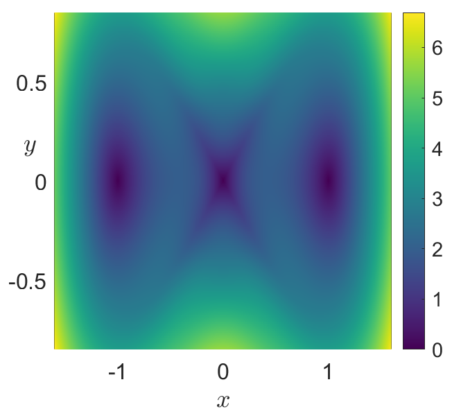
(81)¶\[\begin{equation} \mathcal{W}^{s} = \mathcal{W}^{u} = \left\{(x,y) \in \mathbb{R}^2 \; \Big| \; 2y^2 + x^4 - 2x^2 = 0 \right\} \label{eq:duff_homocMani} \end{equation}\]

Fig. 25 Phase portrait of the autonomous and undamped Duffing oscillator obtained by applying the arclength definition of LDs in Eq. (51) . A) LDs with $\tau = 2$¶

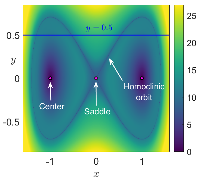
Fig. 26 Phase portrait of the autonomous and undamped Duffing oscillator obtained by applying the arclength definition of LDs in Eq. (51) . B) LDs with $\tau = 10$¶

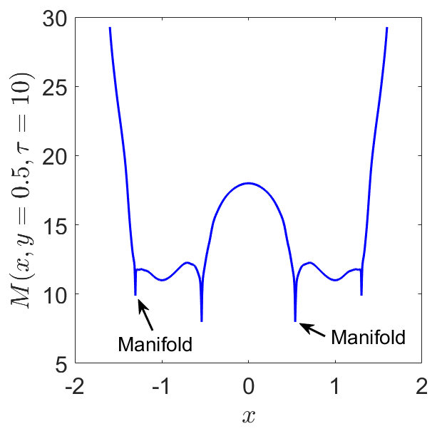
Fig. 27 Phase portrait of the autonomous and undamped Duffing oscillator obtained by applying the arclength definition of LDs in Eq. (51) . C) Value of LDs along the line $y = 0.5$ depicted in panel B) illustrating how the method detects the stable and unstable manifolds at points where the scalar field changes abruptly.¶

We move on to compute LDs for the forced Duffing oscillator. In this situation, the vector field is time-dependent and thus the dynamical system is nonautonomous. The consequence is that the homoclinic connection breaks up and the stable and unstable manifolds intersect, forming an intricate tangle that gives rise to chaos. We illustrate this phenomenon by computing LDs with $\tau = 10$ to reconstruct the phase portrait at the initial time $t_0 = 0$. For the forcing, we use a perturbation strength $\varepsilon = 0.1$, an angular frequency of $\omega = 1$ and a phase $\phi = 0$. This result is shown in Fig. 31 C), and we also depict the forward $(\mathcal{L}^f)$ and backward $(\mathcal{L}^b)$ contributions of LDs in Fig. 31 A) and B) respectively, demonstrating that the method can be used to recover the stable and unstable manifolds separately. Furthermore, by taking the value of LDs along the line $y = 0.5$, the location of the invariant manifolds are highlighted at points corresponding to sharp changes (and local minima) in the scalar field values of LDs.

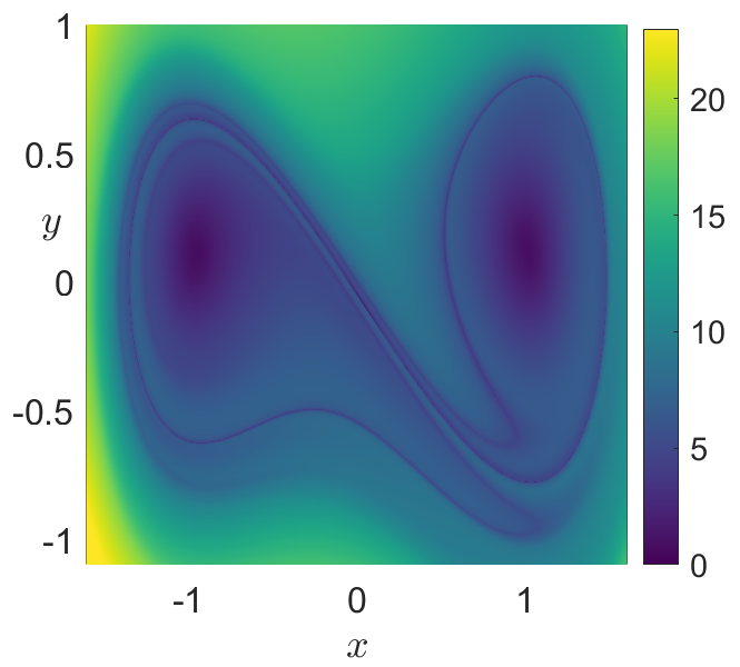
../_images/duffing_stbl_tau_10_pert_01.png

Fig. 28 Phase portrait of the nonautonomous and undamped Duffing oscillator obtained at time $t = 0$ by applying the arclength definition of LDs in Eq. (51) with an integration time $\tau = 10$. A) Forward LDs detect stable manifolds¶

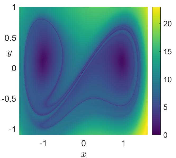
../_images/duffing_unstbl_tau_10_pert_01.png

Fig. 29 Phase portrait of the nonautonomous and undamped Duffing oscillator obtained at time $t = 0$ by applying the arclength definition of LDs in Eq. (51) with an integration time $\tau = 10$. B) Backward LDs highlight unstable manifolds of the system¶

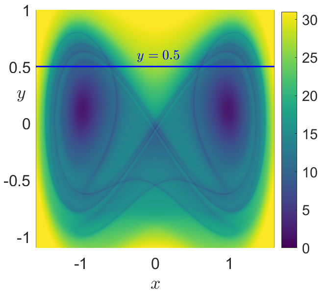
Fig. 30 Phase portrait of the nonautonomous and undamped Duffing oscillator obtained at time $t = 0$ by applying the arclength definition of LDs in Eq. (51) with an integration time $\tau = 10$. C) Total LDs (forward $+$ backward) showing that all invariant manifolds are recovered simultaneously.¶

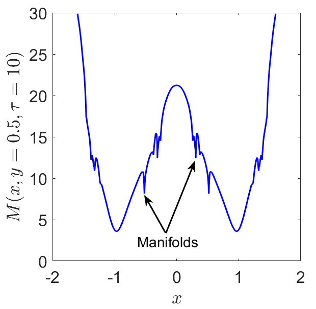
../_images/duffing_maniDetect_pert_01.png

Fig. 31 Phase portrait of the nonautonomous and undamped Duffing oscillator obtained at time $t = 0$ by applying the arclength definition of LDs in Eq. (51) with an integration time $\tau = 10$. D) Value taken by LDs along the line $y = 0.5$ in panel C) to illustrate how the method detects the stable and unstable manifolds at points where the scalar field changes abruptly.¶

The linear Hamiltonian saddle with 2 DoF¶

Consider the two DoF system given by the linear quadratic Hamiltonian associated to an index-1 saddle at the origin. This Hamiltonian and the equations of motion are given by the expressions:

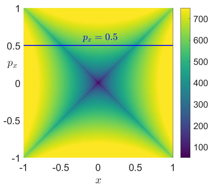
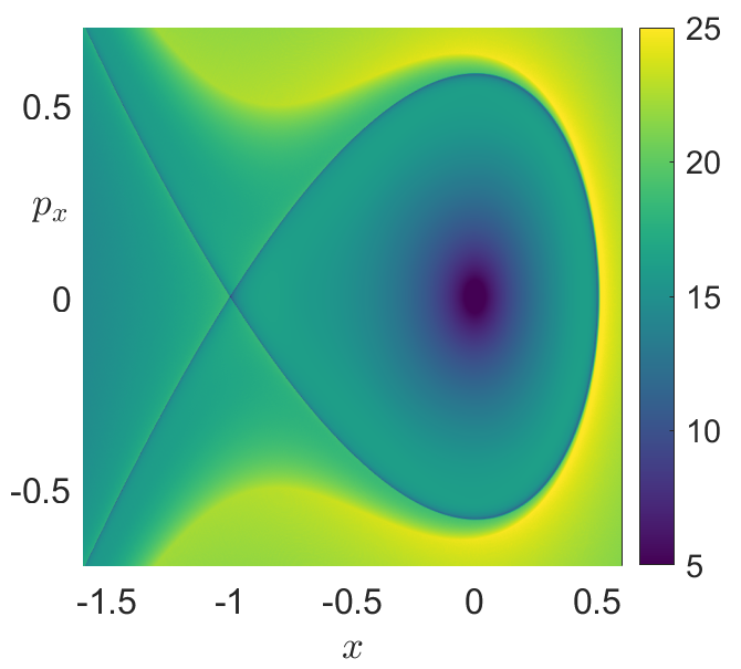
(82)¶\[\begin{split}\begin{eqnarray} H(x,y,p_x,p_y) = \dfrac{\lambda}{2}\left(p_x^2 - x^2\right) + \dfrac{\omega}{2} \left(p_y^2 + y^2 \right) \quad,\quad \begin{cases} \dot{x} = \lambda \, p_x \\ \dot{p}_{x} = \lambda \, x \\ \dot{y} = \omega \, p_y \\ \dot{p}_{y} = -\omega \, y \end{cases} \label{eq:index1_Ham} \end{eqnarray}\end{split}\]

Fig. 32 Phase portrait in the saddle space of the linear Hamiltonian given in Eq. (82). A) Application of the $p$-norm definition of LDs in Eq. (56) using $p = 1/2$ with $\tau = 10$.¶

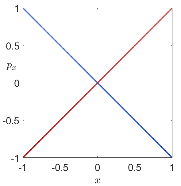
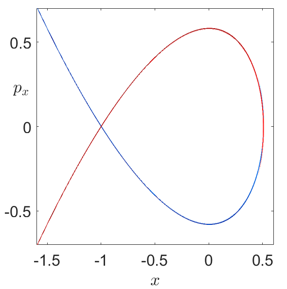
Fig. 33 B) Stable (blue) and unstable (red) invariant manifolds of the unstable periodic orbit at the origin extracted from the gradient of the $M_p$ function.¶

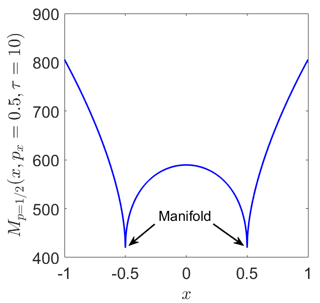
Fig. 34 C) Value of LDs along the line $p_x = 0.5$ depicted in panel A) to illustrate how the method detects the stable and unstable manifolds at points where the scalar field is singular or non-differentiable and attains a local minimum.¶

The Cubic Potential¶

In order to illustrate the issues encountered by the fixed integration time LDs and how the variable integration approach resolves them, we apply the method to a basic one degree-of-freedom Hamiltonian known as the “fish potential”, which is given by the formula:

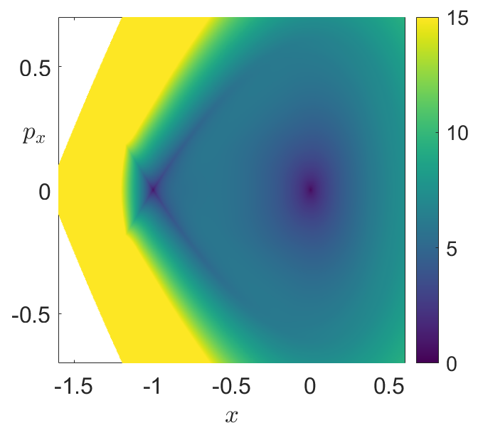
(83)¶\[\begin{split}\begin{equation} H = \dfrac{1}{2} p_x^2 + \dfrac{1}{2} x^2 + \dfrac{1}{3} x^3 \quad \Leftrightarrow \quad \begin{cases} \dot{x} = p_x \\ \dot{p}_{x} = - x - x^2 \end{cases} \;. \label{eq:fish_Ham} \end{equation}\end{split}\]

../_images/LDfixTime_p_05_fishPot_tau_3.png

Fig. 35 Phase portrait of the “fish potential” Hamiltonian in Eq. (83) revealed by the $p$-norm LDs with $p = 1/2$. A) Fixed-time integration LDs in Eq. (56) with $\tau = 3$¶

Fig. 36 Phase portrait of the “fish potential” Hamiltonian in Eq. (83) revealed by the $p$-norm LDs with $p = 1/2$. B) Variable-time integration definition of LDs in Eq. (77) with $\tau = 8$¶

Fig. 37 Phase portrait of the “fish potential” Hamiltonian in Eq. (83) revealed by the $p$-norm LDs with $p = 1/2$. C) Invariant stable (blue) and unstable (red) manifolds of the saddle fixed point extracted from the gradient of the variable time $M_p$ function.¶

The Hénon-Heiles Hamiltonian System¶

We continue illustrating how to apply the method of Lagrangian descriptors to unveil the dynamical skeleton in systems with a high-dimensional phase space by applying this tool to a hallmark Hamiltonian of nonlinear dynamics, the Hénon-Heiles Hamiltonian. This model was introduced in 1964 to study the motion of stars in galaxies [HenonH64] and is described by:

(84)¶\[\begin{split}\begin{equation} H = \dfrac{1}{2} \left(p_x^2 + p_y^2\right) + \dfrac{1}{2}\left(x^2 + y^2\right) + x^2y - \dfrac{1}{3} y^3 \quad \Leftrightarrow \quad \begin{cases} \dot{x} = p_x \\ \dot{p}_{x} = - x - 2xy \\ \dot{y} = p_y \\ \dot{p}_{y} = - y - x^2 + y^2 \end{cases} \;. \label{eq:henon_system} \end{equation}\end{split}\]

which has four equilibrium points: one minimum located at the origin and three saddle-center points at $(0,1)$ and $(\pm \sqrt{3}/2,-1/2)$. The potential energy surface is

\[{ V(x,y) = x^2/2 + y^2/2 + x^2y - y^3/3 }\]

which has a $\pi/3$ rotational symmetry and is characterized by a central scattering region about the origin and three escape channels, see Fig. 39 below for details.

In order to analyze the phase space of the Hénon-Heiles Hamiltonian by means of the variable integration time LDs, we fix an energy $H = H_0$ of the system and choose an interaction region $\mathcal{R}$ defined in configuration space by a circle of radius $15$ centered at the origin. For our analysis we consider the following phase space slices:

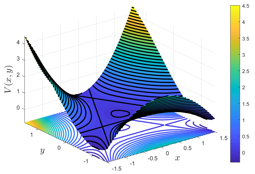
(85)¶\[\begin{split}\begin{eqnarray} \mathcal{U}^{+}_{y,p_y} & = \left\{(x,y,p_x,p_y) \in \mathbb{R}^4 \;|\; H = H_0 \;,\; x = 0 \;,\; p_x > 0\right\} \\[.1cm] \mathcal{V}^{+}_{x,p_x} &= \left\{(x,y,p_x,p_y) \in \mathbb{R}^4 \;|\; H = H_0 \;,\; y = 0 \;,\; p_y > 0\right\} \label{eq:psos} \end{eqnarray}\end{split}\]

Fig. 38 Potential energy surface for the Hénon-Heiles system.¶

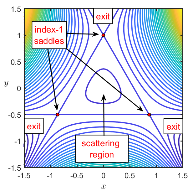
Fig. 39 Potential energy surface projected onto XY plane for the Hénon-Heiles system.¶

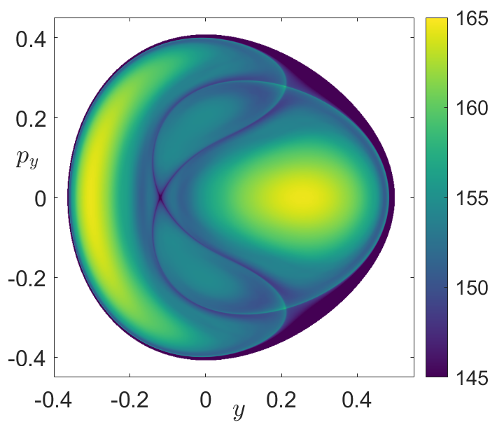
../_images/LDs_Henon_tau_50_x_0_E_1div12.png

Fig. 40 Phase space structures of the Hénon-Heiles Hamiltonian as revealed by the $p$-norm variable integration time LDs with $p = 1/2$. A) LDs computed for $\tau = 50$ in the SOS $\mathcal{U}^{+}_{y,p_y}$ with energy $H = 1/12$¶

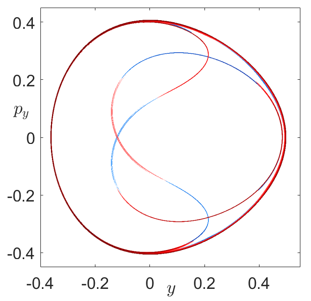
../_images/Mani_Henon_tau_50_x_0_E_1div12.png

Fig. 41 Gradient of the LD function showing stable and unstable manifold intersections in blue and red respectively.¶

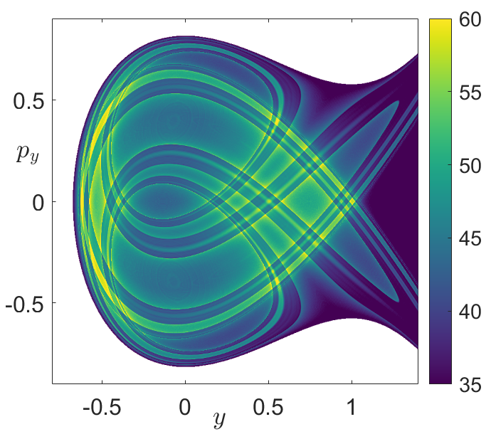
../_images/LDs_Henon_tau_10_x_0_E_1div3.png

Fig. 42 Phase space structures of the Hénon-Heiles Hamiltonian as revealed by the $p$-norm variable integration time LDs with $p = 1/2$. B) LDs for $\tau = 10$ in the SOS $\mathcal{U}^{+}_{y,p_y}$ with energy $H = 1/3$¶

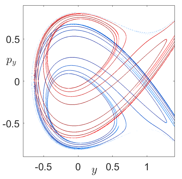
../_images/Mani_Henon_tau_10_x_0_E_1div3.png

Fig. 43 Gradient of the LD function showing stable and unstable manifold intersections in blue and red respectively.¶

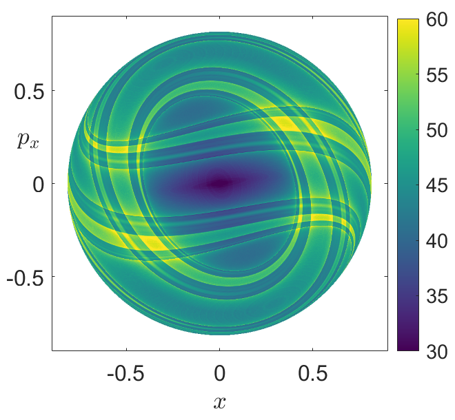
../_images/LDs_Henon_tau_10_y_0_E_1div3.png

Fig. 44 Phase space structures of the Hénon-Heiles Hamiltonian as revealed by the $p$-norm variable integration time LDs with $p = 1/2$. C) LDs for $\tau = 10$ in the SOS $\mathcal{V}^{+}_{x,p_x}$ with energy $H = 1/3$¶

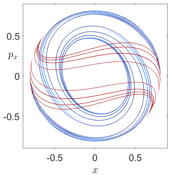
../_images/Mani_Henon_tau_10_y_0_E_1div3.png

Fig. 45 Gradient of the LD function showing stable and unstable manifold intersections in blue and red respectively.¶

Stochastic Lagrangian Descriptors¶

Lagrangian descriptors were extended to stochastic dynamical systems in [BILWM16], and our discussion here is taken from this source, where the reader can also find more details. A basic introduction to stochastic differential equations is in the book [Oks03].

Preliminary concepts¶

Lagrangian descriptors are a trajectory based diagnostic. Therefore we first need to develop the concepts required to describe the nature of trajectories of stochastic differential equations (SDEs). We begin by considering a general system of SDEs expressed in differential form as follows:

(86)¶\[\begin{equation} \label{eq:SDE} dX_{t} = b(X_{t},t)dt + \sigma (X_{t},t)dW_{t}, \quad t \in \mathbb{R}, \end{equation}\]

where $b(\cdot) \in C^{1}(\mathbb{R}^{n}\times \mathbb{R})$ is the deterministic part, $\sigma (\cdot) \in C^{1}(\mathbb{R}^{n}\times \mathbb{R})$ is the random forcing, $W_{t}$ is a Wiener process (also referred to as Brownian motion) whose definition we give later, and $X_{t}$ is the solution of the equation. All these functions take values in $\mathbb{R}^{n}$.

As the notion of solution of a SDE is closely related with the Wiener process, we state what is meant by $W(\cdot )$. This definition is given in [Dua15], and this reference serves to provide the background for all of the notions in this section. Also, throughout we will use $\Omega$ to denote the probability space where the Wiener process is defined.

Definition Wiener/Brownian process

A real valued stochastic Wiener or Brownian process $W(\cdot)$ is a stochastic process defined in a probability space $(\Omega , {\cal F},{\cal P})$ which satisfies

$W_0 = 0$ (standard Brownian motion),
$W_t - W_s$ follows a Normal distribution $N(0,t-s)$ for all $t\geq s \geq 0$,
for all time $0 < t_1 < t_2 < ... < t_n$, the random variables $W_{t_1}, W_{t_2} - W_{t_1},... , W_{t_n} - W_{t_{n-1}}$ are independent (independent increments).

Moreover, $W(\cdot)$ is a real valued two-sided Wiener process if conditions (ii) and (iii) change into

$W_t - W_s$ follows a Normal distribution $N(0,|t-s|)$ for all $t, s \in \mathbb{R}$,
for all time $t_1 , t_2 , ... , t_{2n} \in \mathbb{R}$ such that the intervals $\lbrace (t_{2i-1},t_{2i}) \rbrace_{i=1}^{n}$ are non-intersecting between them (Note), the random variables $W_{t_1}-W_{t_2}, W_{t_3} - W_{t_4},... , W_{t_{2n-1}} - W_{t_{2n}}$ are independent.

This method of Lagrangian descriptors has been developed for deterministic differential equations whose temporal domain is $\mathbb{R}$. In this sense it is natural to work with two-sided solutions as well as two-sided Wiener processes. Henceforth, every Wiener process $W(\cdot )$ considered in the this article will be of this form.

Given that any Wiener process $W(\cdot )$ is a stochastic process, by definition this is a family of random real variables $\lbrace W_{t}, t\in \mathbb{R} \rbrace$ in such a way that for each $\omega \in \Omega$ there exists a mapping, $ t \longmapsto W_{t}(\omega )$, known as the trajectory of a Wiener process.

Analogously to the Wiener process, the solution $X_{t}$ of the SDE (86) is also a stochastic process. In particular, it is a family of random variables $\lbrace X_{t}, t\in \mathbb{R} \rbrace$ such that for each $\omega \in \Omega$, the trajectory of $X_{t}$ satisfies

(87)¶\[\begin{equation} \label{Xt} t \longmapsto X_{t}(\omega ) = X_{0}(\omega ) + \int_{0}^{t} b(X_{s}(\omega ), s)ds + \int_{0}^{t} \sigma (X_{s}(\omega ), s)dW_{s}(\omega ), \end{equation}\]

where $X_{0}:\Omega \rightarrow \mathbb{R}^{n}$ is the initial condition. In addition, as $b(\cdot)$ and $\sigma(\cdot)$ are smooth functions, they are locally Lipschitz and this leads to existence and pathwise uniqueness of a local, continuous solution (see [Dua15]). That is if any two stochastic processes $X^1$ and $X^2$ are local solutions in time of SDE (86) , then $X^1_t(\omega) = X^2_t(\omega)$ over a time interval $t \in (t_{i},t_{f})$ and for almost every $\omega \in \Omega$.

At each instant of time $t$, the deterministic integral $\int_{0}^{t} b(X_{s}(\omega ))ds$ is defined by the usual Riemann integration scheme since $b$ is assumed to be a differentiable function. However, the stochastic integral term is chosen to be defined by the It^{o} integral scheme:

(88)¶\[\begin{equation} \label{Ito} \int_{0}^{t} \sigma (X_{s}(\omega ),s)dW_{s}(\omega ) = \lim_{N \rightarrow \infty} \sum_{i=0}^{N-1} \sigma (X_{i\frac{t}{N}}(\omega ), it/N) \cdot \left[ W_{(i+1)\frac{t}{N}}(\omega ) - W_{i\frac{t}{N}}(\omega ) \right]. \end{equation}\]

This scheme will also facilitate the implementation of a numerical method for computing approximations for the solution $X_{t}$ in the next section.

Once the notion of solution, $X_{t}$, of a SDE (86) is established, it is natural to ask if the same notions and ideas familiar from the study of deterministic differential equations from the dynamical systems point of view are still valid for SDEs. In particular, we want to consider the notion of hyperbolic trajectory and its stable and unstable manifolds in the context of SDEs. We also want to consider how such notions would manifest themselves in the context of phase space transport for SDEs, and the stochastic Lagrangian descriptor will play a key role in considering these questions from a practical point of view.

We first discuss the notion of an invariant set for a SDE. In the deterministic case the simplest possible invariant set is a single trajectory of the differential equation. More precisely, it is the set of points through which a solution passes. Building on this construction, an invariant set is a collection of trajectories of different solutions. This is the most basic way to characterize the invariant sets with respect to a deterministic differential equation of the form

(89)¶\[\begin{equation} \label{deterministic_system} \dot{x} = f(x,t), \quad x \in \mathbb{R}^{n}, \quad t \in \mathbb{R}. \end{equation}\]

For verifying the invariance of such sets the solution mapping generated by the vector field is used. For deterministic autonomous systems these are referred to as flows (or “dynamical systems”) and for deterministic nonautonomous systems they are referred to as processes. The formal definitions can be found in [KR11].

A similar notion of solution mapping for SDEs is introduced using the notion of a random dynamical system $\varphi$ (henceforth referred to as RDS) in the context of SDEs. This function $\varphi$ is also a solution mapping of a SDE that satisfies several conditions, but compared with the solution mappings in the deterministic case, this RDS depends on an extra argument which is the random variable $\omega \in \Omega$. Furthermore the random variable $\omega$ evolves with respect to $t$ by means of a dynamical system $\lbrace \theta_{t} \rbrace_{t \in \mathbb{R}}$ defined over the probability space $\Omega$.

Definition Random Dynamical System

Note

Given the probability measure $\mathcal{P}$ associated with the space $(\Omega , \mathcal{F},\mathcal{P})$, this remains invariant under the dynamical system $\lbrace \theta_{t} \rbrace_{t \in \mathbb{R}}$. Formally, $\theta_{t}\mathcal{P} = \mathcal{P}$ for every $t \in \mathbb{R}$. This statement means that $\mathcal{P}(B)=\mathcal{P}(\theta_{t}(B))$ for every $t \in \mathbb{R}$ and every subset $B \in \mathcal{F}$. Indeed for any dynamical system $\lbrace \theta_{t} \rbrace_{t \in \mathbb{R}}$ defined over the same probability space $\Omega$ as a Wiener process $W(\cdot )$, we have the equality $W_{s}(\theta_{t}\omega ) = W_{t+s}(\omega )-W_{t}(\omega )$ which implies that $dW_{s}(\theta_{t}\omega ) = dW_{t+s}(\omega )$ for every $s,t \in \mathbb{R}$ (see [Dua15] for a detailed explanation).

Let $\lbrace \theta_{t} \rbrace_{t \in \mathbb{R}}$ be a measure-preserving (Note) dynamical system defined over $\Omega$, and let $\varphi : \mathbb{R} \times \Omega \times \mathbb{R}^{n} \rightarrow \mathbb{R}^{n}$ be a measurable mapping such that $(t,\cdot , x) \mapsto \varphi (t,\omega ,x)$ is continuous for all $\omega \in \Omega$, and the family of functions $\lbrace \varphi (t,\omega ,\cdot ): \mathbb{R}^{n} \rightarrow \mathbb{R}^{n} \rbrace$ has the cocycle property:

\[ \varphi (0,\omega ,x)=x \quad \text{and} \quad \varphi (t+s,\omega ,x) = \varphi(t,\theta_{s}\omega,\varphi (s,\omega ,x)) \quad \text{for all } t,s \in \mathbb{R}, \text{ } x \in \mathbb{R}^{n} \text{ and } \omega \in \Omega .\]

Then the mapping $\varphi$ is a random dynamical system with respect to the stochastic differential equation

\begin{equation*} dX_{t} = b(X_{t})dt + \sigma (X_{t})dW_{t} \end{equation*}

if $\varphi (t,\omega ,x)$ is a solution of the equation.

Analogous to the deterministic case, the definition of invariance with respect to a SDE can be characterized in terms of a RDS. This is an important topic in our consideration of stochastic Lagrangian descriptors. Now we introduce an example of a SDE for which the analytical expression of the RDS is obtained. This will be a benchmark example in our development of stochastic Lagrangian descriptors their relation to stochastic invariant manifolds.

Noisy saddle point

For the stochastic differential equation

(90)¶\[\begin{split}\begin{equation} \label{noisy_saddle} \begin{cases} dX_{t} = X_{t}dt + dW_{t}^{1} \\ dY_{t} = -Y_{t}dt + dW_{t}^{2} \end{cases} \end{equation}\end{split}\]

where $W_{t}^{1}$ and $W_{t}^{2}$ are two different Wiener processes, the solutions take the expressions

(91)¶\[\begin{equation} \label{noisy_saddle_solutions} X_{t} = e^{t} \left( X_{0}(\omega ) + \int_{0}^{t}e^{-s}dW_{s}^{1}(\omega ) \right) \quad , \quad Y_{t} = e^{-t} \left( Y_{0}(\omega ) + \int_{0}^{t}e^{s}dW_{s}^{2}(\omega ) \right) \end{equation}\]

and therefore the random dynamical system $\varphi$ takes the form

(92)¶\[\begin{split}\begin{equation} \label{noisy_saddle_RDS} \begin{array}{ccccccccc} \varphi : & & \mathbb{R} \times \Omega \times \mathbb{R}^{2} & & \longrightarrow & & \mathbb{R}^{2} & & \\ & & (t,\omega ,(x,y)) & & \longmapsto & & \left( \varphi_{1}(t,\omega ,x),\varphi_{2}(t,\omega ,y) \right) & = & \left( e^{t} \left( x + \int_{0}^{t}e^{-s}dW_{s}^{1}(\omega ) \right) , e^{-t} \left( y + \int_{0}^{t}e^{s}dW_{s}^{2}(\omega ) \right) \right) . \end{array} \end{equation}\end{split}\]

Notice that this last definition Random Dynamical System is expressed in terms of SDEs with time-independent coefficients $b,\sigma$. For more general SDEs a definition of nonautonomous RDS is developed in [Dua15]. However, for the remaining examples considered in this article we make use of the already given definition of RDS.

Once we have the notion of RDS, it can be used to describe and detect geometrical structures and determine their influence on the dynamics of trajectories. Specifically, in clear analogy with the deterministic case, we focus on those trajectories whose expressions do not depend explicitly on time $t$, which are referred as random fixed points. Moreover, their stable and unstable manifolds, which may also depend on the random variable $\omega$, are also objects of interest due to their influence on the dynamical behavior of nearby trajectories. Both types of objects are invariant. Therefore we describe a characterization of invariant sets with respect to a SDE by means of an associated RDS.

Definition Invariant Set

A non empty collection $M : \Omega \rightarrow \mathcal{P}(\mathbb{R}^{n})$, where $M(\omega ) \subseteq \mathbb{R}^{n}$ is a closed subset for every $\omega \in \Omega$, is called an invariant set for a random dynamical system $\varphi$ if

(93)¶\[\begin{equation} \label{invariance} \varphi (t,\omega ,M(\omega )) = M(\theta_{t}\omega ) \quad \text{for every } t \in \mathbb{R} \text{ and every } \omega \in \Omega. \end{equation}\]

Again, we return to the noisy saddle (90) , which is an example of a SDE for which several invariant sets can be easily characterized by means of its corresponding RDS.

Noisy saddle point

For the stochastic differential equations

(94)¶\[\begin{split}\begin{equation} \begin{cases} dX_{t} = X_{t}dt + dW_{t}^{1} \\ dY_{t} = -Y_{t}dt + dW_{t}^{2} \end{cases} \end{equation}\end{split}\]

where $W_{t}^{1}$ and $W_{t}^{2}$ are two different Wiener processes, the solution mapping $\varphi$ is given by the following expression

(95)¶\[\begin{split}\begin{equation} \begin{array}{ccccccccc} \varphi : & & \mathbb{R} \times \Omega \times \mathbb{R}^{2} & & \longrightarrow & & \mathbb{R}^{2} & & \\ & & (t,\omega ,(x,y)) & & \longmapsto & & (\varphi_{1}(t,\omega ,x),\varphi_{2}(t,\omega ,y)) & = & \left( e^{t} \left( x + \int_{0}^{t}e^{-s}dW_{s}^{1}(\omega ) \right) , e^{-t} \left( y + \int_{0}^{t}e^{s}dW_{s}^{2}(\omega ) \right) \right) . \end{array} \end{equation}\end{split}\]

Notice that this is a decoupled random dynamical system. There exists a solution whose components do not depend on variable $t$ and are convergent for almost every $\omega \in \Omega$ as a consequence of the properties of Wiener processes (see [Dua15]). This solution has the form: $$\tilde{X}(\omega) = (\tilde{x}(\omega ),\tilde{y}(\omega )) = \left( - \int_{0}^{\infty}e^{-s}dW_{s}^{1}(\omega ) , \int_{-\infty}^{0}e^{s}dW_{s}^{2}(\omega ) \right) .$$ Actually, $\tilde{X}(\omega )$ is a solution because it satisfies the invariance property that we now verify:

(96)¶\[\begin{split}\begin{equation} \label{invariance_x} \begin{array}{ccl} \varphi_{1} (t,\omega ,\tilde{x}(\omega )) & = & \displaystyle{e^{t}\left( -\int_{0}^{+\infty}e^{-s}dW^{1}_{s}(\omega ) + \int_{0}^{t}e^{-s}dW^{1}_{s}(\omega ) \right) } = \displaystyle{-\int_{t}^{+\infty}e^{-(s-t)}dW^{1}_{s}(\omega ) }\\ & = & \displaystyle{-\int_{0}^{+\infty}e^{-t'}dW^{1}_{t'+t}(\omega) = - \int_{0}^{+\infty}e^{-t'}dW^{1}_{t'}(\theta_{t}\omega ) = \tilde{x}(\theta_{t}\omega )} \quad \text{by means of } t'=s-t, \end{array} \end{equation}\end{split}\]

(97)¶\[\begin{split}\begin{equation} \label{invariance_y} \begin{array}{lll} \varphi_{2} (t,\omega ,\tilde{y}(\omega )) & = & \displaystyle{e^{-t}\left( \int_{-\infty}^{0}e^{s}dW^{2}_{s}(\omega ) + \int_{0}^{t}e^{s}dW^{2}_{s}(\omega ) \right) = \int_{-\infty}^{t}e^{s-t}dW^{2}_{s}(\omega ) = \int_{-\infty}^{0}e^{t'}dW^{2}_{t'+t}(\omega )} \\ & = & \displaystyle{ \int_{-\infty}^{0}e^{t'}dW^{2}_{t'}(\theta_{t}\omega ) = \tilde{y}(\theta_{t}\omega )} \quad \text{by means of } t'=s-t. \end{array} \end{equation}\end{split}\]

This implies that $\varphi (t,\omega ,\tilde{X}(\omega )) = \tilde{X}(\theta_{t} \omega)$ for every $t \in \mathbb{R}$ and every $\omega \in \Omega$. Therefore $\tilde{X}(\omega )$ satisfies the invariance property (93). This conclusion comes from the fact that $\tilde{x}(\omega )$ and $\tilde{y}(\omega )$ are also invariant under the components $\varphi_{1}$ and $\varphi_{2}$, in case these are seen as separate RDSs defined over $\mathbb{R}$ (see (96) and eq:invariance_y, respectively).

Due to its independence with respect to the time variable $t$, it is said that $\tilde{X}(\omega )$ is a random fixed point of the SDE (90), or more commonly a stationary orbit. As the trajectory of $\tilde{X}(\omega )$ (and separately its components $\tilde{x}(\omega )$ and $\tilde{y}(\omega )$) is proved to be an invariant set, it is straightforward to check that the two following subsets of $\mathbb{R}^{2}$,

\[\mathcal{S}(\omega ) = \lbrace (x,y) \in \mathbb{R}^{2} : x = \tilde{x}(\omega ) \rbrace \quad , \quad \mathcal{U}(\omega ) = \lbrace (x,y) \in \mathbb{R}^{2} : y = \tilde{y}(\omega ) \rbrace \]

are also invariant with respect to the RDS $\varphi$. Similarly to the deterministic setting, these are referred to as the stable and unstable manifolds of the stationary orbit respectively. Additionally, in order to prove the separating nature of these two manifolds and the stationary orbit with respect to their nearby trajectories, let’s consider any other solution $(\overline{x}_{t},\overline{y}_{t})$ of the noisy saddle with initial conditions at time $t=0$,

(98)¶\[\begin{equation} \overline{x}_{0} = \tilde{x}(\omega ) + \epsilon_{1}(\omega ) , \quad \overline{y}_{0} = \tilde{y}(\omega ) + \epsilon_{2}(\omega ), \quad \text{being } \epsilon_{1}(\omega ), \epsilon_{2}(\omega ) \text{ two random variables.} \end{equation}\]

If the corresponding RDS $\varphi$ is applied to compare the evolution of this solution $(\overline{x}_{t},\overline{y}_{t})$ and the stationary orbit, there arises an exponential dichotomy:

\[ (\overline{x}_{t},\overline{y}_{t}) - (\tilde{x}(\theta_{t}\omega ),\tilde{y}(\theta_{t}\omega )) = \varphi (t,\omega ,(\overline{x}_{0},\overline{y}_{0})) - \varphi (t,\omega ,(\tilde{x}(\omega ),\tilde{y}(\omega ))) \]

\[= \left( e^{t}\left[ \overline{x}_{0} + \int_{0}^{t}e^{-s}dW_{s}^{1}(\omega ) - \tilde{x}(\omega ) - \int_{0}^{t}e^{-s}dW_{s}^{1}(\omega ) \right] , e^{-t}\left[ \overline{y}_{0} + \int_{0}^{t}e^{s}dW_{s}^{2}(\omega ) - \tilde{y}(\omega ) - \int_{0}^{t}e^{s}dW_{s}^{2}(\omega ) \right] \right) \]

(99)¶\[\begin{equation} = \left( e^{t} \left( \tilde{x}(\omega )+\epsilon_{1}(\omega )-\tilde{x}(\omega ) \right) ,e^{-t} \left( \tilde{y}(\omega )+\epsilon_{2}(\omega )-\tilde{y}(\omega ) \right) \right) = \left( \epsilon_{1}(\omega )e^{t},\epsilon_{2}(\omega )e^{-t} \right) . \end{equation}\]

Considering that $(\overline{x}_{t},\overline{y}_{t})$ is different from $(\tilde{x}(\omega ),\tilde{y}(\omega ))$ then one of the two cases $\epsilon_{1} \not \equiv 0$ or $\epsilon_{2} \not \equiv 0$ holds, let say $\epsilon_{1} \not = 0$ or $\epsilon_{2} \not = 0$ for almost every $\omega \in \Omega$. In the first case, the distance between both trajectories $(\overline{x}_{t},\overline{y}_{t})$ and $(\tilde{x},\tilde{y})$ increases at an exponential rate in positive time:

(100)¶\[\begin{equation} \label{eq:eq_1} \Vert \varphi (t,\omega ,(\overline{x}_{t},\overline{y}_{t}))-\varphi (t,\omega ,(\tilde{x},\tilde{y})) \Vert \geq |\epsilon_{1}(\omega )e^{t} | \longrightarrow + \infty \quad \text{when } t \rightarrow + \infty \text{ and for a.e. } \omega \in \Omega . \end{equation}\]

Similarly to this case, when the second option holds the distance between both trajectories increases at a exponential rate in negative time. It does not matter how close the initial condition $(\overline{x}_{0},\overline{x}_{0})$ is from $(\tilde{x}(\omega ),\tilde{y}(\omega ))$ at the initial time $t=0$. Actually this same exponentially growing separation can be achieved for any other initial time $t \not = 0$. Following these arguments, one can check that the two manifolds $\mathcal{S}(\omega )$ and $\mathcal{U}(\omega )$ also exhibit this same separating behaviour as the stationary orbit. Moreover, we remark that almost surely the stationary orbit is the only solution whose components are bounded.

These facts highlight the distinguished nature of the stationary orbit (and its manifolds) in the sense that it is an isolated solution from the others. Apart from the fact that $(\tilde{x},\tilde{y})$ “moves” in a bounded domain for every $t \in \mathbb{R}$, any other trajectory eventually passing through an arbitrary neighborhood of $(\tilde{x},\tilde{y})$ at any given instant of time $t$, leaves the neighborhood and then separates from the stationary orbit in either positive or negative time. Specifically, this separation rate is exponential for the noisy saddle, just in the same way as for the deterministic saddle.

These features are also observed for the trajectories within the stable and unstable manifolds of the stationary orbit, but in a more restrictive manner than $(\tilde{x},\tilde{y})$. Taking for instance an arbitrary trajectory $(x^{s},y^{s})$ located at $\mathcal{S}(\omega )$ for every $t \in \mathbb{R}$, its first component $x^{s}_{t}=\tilde{x}(\omega )$ remains bounded for almost every $\omega \in \Omega$. In contrast, any other solution passing arbitrarily closed to $(x^{s},y^{s})$ neither being part of $\mathcal{S}(\omega )$ nor being the stationary orbit, satisfies the previous inequality (100) and therefore separates from $\mathcal{S}(\omega )$ at an exponential rate for increasing time. With this framework we can now introduce the formal definitions of stationary orbit and invariant manifold.

Definition Stationary Orbit

A random variable $\tilde{X}: \Omega \rightarrow \mathbb{R}^{n}$ is called a stationary orbit (random fixed point) for a random dynamical system $\varphi$ if

\[\varphi(t, \omega, \tilde{X}(\omega)) = \tilde{X}(\theta_t\omega), \quad \text{for every } t \in \mathbb{R} \text{ and every } \omega \in \Omega .\]

Obviously every stationary orbit $\tilde{X}(\omega )$ is an invariant set with respect to a RDS as it satisfies Definition Invariant Set. Among several definitions of invariant manifolds given in the bibliography (for example [arno98], [boxl89], [Dua15]), which have different formalisms but share the same philosophy, we choose the one given in [Dua15] because it adapts to our example in a very direct way.

Definition

A random invariant set $M: \Omega \rightarrow \mathcal{P}(\mathbb{R}^{n})$ for a random dynamical system $\varphi$ is called a $C^{k}$-Lipschitz invariant manifold if it can be represented by a graph of a $C^{k}$ Lipschitz mapping ($k \geq 1$)

\[\begin{equation*} \gamma (\omega , \cdot ):H^{+} \to H^{-}, \quad \text{with direct sum decomposition } H^{+} \oplus H^{-} = \mathbb{R}^{n} \end{equation*}\]

such that

\[\begin{equation*} \quad M(\omega ) = \lbrace x^{+} \oplus \gamma(\omega ,x^{+}) : x^{+} \in H^{+} \rbrace \quad \text{for every } \omega \in \Omega. \end{equation*}\]

This is a very limited notion of invariant manifold as its formal definition requires the set to be represented by a Lipschitz graph. Anyway, it is consistent with the already established manifolds $\mathcal{S}(\omega )$ and $\mathcal{U}(\omega )$ as these can be represented as the graphs of two functions $\gamma_{s}$ and $\gamma_{u}$ respectively,

\[\begin{split}\begin{align*} \begin{array}{ccccc} \gamma_{s} (\omega , \cdot ) & : & span \lbrace \left( \begin{array}{c} 0 \\ 1 \end{array} \right) \rbrace & \longrightarrow & span \lbrace \left( \begin{array}{c} 1 \\ 0 \end{array} \right) \rbrace \\ & & \left( \begin{array}{c} 0 \\ t \end{array} \right) & \longmapsto & \left( \begin{array}{c} \tilde{x}(\omega ) \\ 0 \end{array} \right) \end{array} \; \text{and} \; \begin{array}{ccccc} \gamma_{u} (\omega , \cdot ) & : & span \lbrace \left( \begin{array}{c} 1 \\ 0 \end{array} \right) \rbrace & \longrightarrow & span \lbrace \left( \begin{array}{c} 0 \\ 1 \end{array} \right) \rbrace \\ & & \left( \begin{array}{c} t \\ 0 \end{array} \right) & \longmapsto & \left( \begin{array}{c} 0 \\ \tilde{y}(\omega ) \end{array} \right) \quad . \end{array} \end{align*}\end{split}\]

Actually the domains of such functions $\gamma_{s}$ and $\gamma_{u}$ are the linear subspaces $E^{s}(\omega )$ and $E^{u}(\omega )$, known as the stable and unstable subspaces of the random dynamical system $\Phi (t,\omega )$. This last mapping is obtained from linearizing the original RDS $\varphi$ over the stationary orbit $(\tilde{x},\tilde{y})$. This result serves as an argument to denote $\mathcal{S}(\omega )$ and $\mathcal{U}(\omega )$ as the stable and unstable manifolds of the stationary orbit, not only because these two subsets are invariant under $\varphi$, as one can deduce from (96) and (96), but also due to the dynamical behaviour of their trajectories in a neighborhood of the stationary orbit $\tilde{X}(\omega )$. Hence the important characteristic of $\tilde{X}(\omega )=(\tilde{x},\tilde{y})$ is not only its independence with respect to the time variable $t$; but also the fact that it exhibits hyperbolic behaviour with respect to its neighboring trajectories. Considering the hyperbolicity of a given solution, as well as in the deterministic context, means considering the hyperbolicity of the RDS $\varphi$ linearized over such solution. Specifically, the Oseledets’ multiplicative ergodic theorem for random dynamical systems ([arno98] and [Dua15]) ensures the existence of a Lyapunov spectrum which is necessary to determine whether the stationary orbit $\tilde{X}(\omega )$ is hyperbolic or not. All these issues are well reported in [Dua15], including the proof that the noisy saddle (90) satisfies the Oseledets’ multiplicative ergodic theorem conditions.

Before implementing the numerical method of Lagrangian descriptors to several examples of SDEs, it is important to remark why random fixed points and their respective stable and unstable manifolds govern the nearby trajectories, and furthermore, how they may influence the dynamics throughout the rest of the domain. These are essential issues in order to describe the global phase space motion of solutions of SDEs. However, these questions do not have a simple answer. For instance, in the noisy saddle example (90) the geometrical structures arising from the dynamics generated around the stationary orbit are quite similar to the dynamics corresponding to the deterministic saddle point $\lbrace \dot{x}=x,\dot{y}=-y \rbrace$. Significantly, the manifolds $\mathcal{S}(\omega )$ and $\mathcal{U}(\omega )$ of the noisy saddle form two dynamical barriers for other trajectories in the same way that the manifolds $\lbrace x = 0 \rbrace$ and $\lbrace y = 0 \rbrace$ of the deterministic saddle work. This means that for any particular experiment, i.e., for any given $\omega \in \Omega$, the manifolds $\mathcal{S}(\omega )$ and $\mathcal{U}(\omega )$ are determined and cannot be “crossed” by other trajectories due to the uniqueness of solutions (remember that the manifolds are invariant under the RDS (92) and are comprised of an infinite family of solutions). Also by considering the exponential separation rates reported in (100) with the rest of trajectories, the manifolds $\mathcal{S}(\omega )$ and $\mathcal{U}(\omega )$ divide the plane $\mathbb{R}^{2}$ of initial conditions into four qualitatively distinct dynamical regions; therefore providing a phase portrait representation.

Note

Otherwise, if nonlinearity is dominating the behavior of the terms in equation (86) then the correspondence between the manifolds for $\Phi (t, \omega )$ to the manifolds for $\varphi$ needs to be made by means of the local stable and unstable manifold theorem (see [moham99], Theorem 3.1). Therein it is considered a homeomorphism $H(\omega )$ which establishes the equivalence of the geometrical structures arising for both sets of manifolds, and as a consequence the manifolds for $\varphi$ inherit the same dynamics as the ones for $\Phi (t, \omega )$ but only in a neighborhood of the stationary orbit. In this sense the existence of such manifolds for a nonlinear RDS $\varphi$ is only ensured locally. Anyway this result provides a very good approximation to the stochastic dynamics of a system, and enables us to discuss the different patterns of behavior of the solutions in the following examples.

Nevertheless it remains to show that such analogy can be found between other SDEs and their corresponding non-noisy deterministic differential equations (Note). In this direction there is a recent result ([CDW16], Theorem 2.1) which ensures the equivalence in the dynamics of both kinds of equations when the noisy term $\sigma$ is additive (i.e., $\sigma$ does not depend on the solution $X_{t}$). Although this was done by means of the most probable phase portrait, a technique that closely resembles the ordinary phase space for deterministic systems, this fact might indicate that such analogy in the dynamics cannot be achieved when the noise does depend explicitly on the solution $X_{t}$. Actually any additive noise affects all the particles together at the same magnitude.

Anyway the noisy saddle serves to establish an analogy to the dynamics with the deterministic saddle. One of its features is the contrast between the growth of the components $X_{t}$ and $Y_{t}$, which mainly have a positive and negative exponential growth respectively. We will see that this is graphically captured when applying the stochastic Lagrangian descriptors method to the SDE (90) over a domain of the stationary orbit. Moreover when representing the stochastic Lagrangian descriptor values for the noisy saddle, one can observe that the lowest values are precisely located on the manifolds $\mathcal{S}(\omega )$ and $\mathcal{U}(\omega )$. These are manifested as sharp features indicating a rapid change of the values that the stochastic Lagrangian descriptor assumes. This geometrical structure formed by “local minimums” has a very marked crossed form and it is straightforward to think that the stationary orbit is located at the intersection of the two cross-sections. These statements are supported afterwards by numerical simulations and analytical results.

The stochastic Lagrangian descriptor¶

The definition of stochastic Lagrangian descriptors that we introduce here is based on the discretization of the continuous time definition given in Eq. (56) that relies on the computation of the $p$-norm of trajectories. In fact, this discretization gave rise to a version of LDs that can be used to analyze discrete time dynamical systems (maps), see [LBIWMancho15]. Let $\{x_i\}^{N}_{i = -N}$ denote an orbit of $(2N + 1)$ points, where $x_i \in \mathbb{R}^n$ and $N \in \mathbb{N}$ is the number of iterations of the map. Considering the space of orbits as a sequence space, the discrete Lagrangian descriptor was defined in terms of the $\ell^p$-norm of an orbit as follows:

(101)¶\[\begin{equation} \displaystyle{MD_p(x_0, N) = \sum^{N-1}_{i = -N}\Vert x_{i+1} - x_i \Vert_p, \quad p \leq 1.} \end{equation}\]

This alternative definition allows us to prove formally the non-differentiability of the $MD_p$ function through points that belong to invariant manifolds of a hyperbolic trajectory. This fact implies a better visualization of the invariant manifolds as they are detected over areas where the $MD_p$ function presents abrupt changes in its values.

Now we extend these ideas to the context of stochastic differential equations. For this purpose we consider a general SDE of the form:

(102)¶\[\begin{equation} dX_t = b(X_t, t)dt + \sigma(X_t, t)dW_t, \quad X_{t_0} = x_0, \label{eq:stochastic_lagrangian_system} \end{equation}\]

where $X_t$ denotes the solution of the system, $b(\cdot)$ and $\sigma(\cdot)$ are Lipschitz functions which ensure uniqueness of solutions and $W_t$ is a two-sided Wiener process. Henceforth, we make use of the following notation

(103)¶\[\begin{equation} X_{t_j} := X_{t_0+j\Delta t}, \end{equation}\]

for a given $\Delta t>0$ small enough and $j=-N,\cdots ,-1,0,1, \cdots ,N$.

Definition

The stochastic Lagrangian descriptor evaluated for SDE (102) with general solution $\textbf{X}_{t}(\omega )$ is given by

(104)¶\[\begin{equation} MS_p(\textbf{x}_0, t_0, \tau, \omega) = \sum^{N-1}_{i = -N} \Vert \textbf{X}_{t_{i+1}} - \textbf{X}_{t_i} \Vert_p \label{eq:MS} \end{equation}\]

where $\lbrace \textbf{X}_{t_{j}} \rbrace_{j=-N}^{N}$ is a discretization of the solution such that $\textbf{X}_{t_{-N}} = \textbf{X}_{-\tau}$, $\textbf{X}_{t_N} = \textbf{X}_{\tau}$, $\textbf{X}_{t_0} = \textbf{x}_{0}$, for a given $\omega \in \Omega$.

Definition

Obviously every output of the $MS_p$ function highly depends on the experiment $\omega \in \Omega$ where $\Omega$ is the probability space that includes all the possible outcomes of a given phenomena. Therefore in order to analyze the homogeneity of a given set of outputs, we consider a sequence of results of the $MS_p$ function for the same stochastic equation (102) : $MS_p(\cdot, \omega_1)$, $MS_p(\cdot, \omega_2)$, $\cdots$, $MS_p(\cdot, \omega_M)$. It is feasible that the following relation holds

(105)¶\[\begin{equation} d(MS_p(\cdot, \omega_i), MS_p(\cdot, \omega_j)) < \delta, \quad \text{for all } i,j, \label{eq:deterministic_tol} \end{equation}\]

where $d$ is a metric that measures the similarity between two matrices (for instance the Frobenius norm $\Vert A-B \Vert_F = \sqrt{Tr((A-B)\cdot (A-B)^T)}$) and $\delta$ is a positive tolerance. Nevertheless for general stochastic differential equations, expression (105) does not usually hold. Alternatively if the elements of the sequence of matrices $MS_p(\cdot, \omega_1)$, $MS_p(\cdot, \omega_2)$, $\cdots$, $MS_p(\cdot, \omega_M)$ do not have much similarity to each other, it may be of more use to define the mean of the outputs

(106)¶\[\begin{equation} \displaystyle{\mathbb{E} \left[ MS_p(\cdot, \omega) \right] = \left( \frac{MS_p(\cdot, \omega_1) + MS_p(\cdot, \omega_2) + \cdots + MS_p(\cdot, \omega_M)}{M}\right) ,} \label{eq:mean_MSp_value} \end{equation}\]

Numerical Simulation of the Stochastic Lagrangian Descriptor¶

In this section we describe the stochastic Lagrangian descriptor method that can be used to numerically solve and visualize the geometrical structures of SDEs. Consider a general $n$-dimensional SDE of the form

(107)¶\[\begin{equation} dX^j_t = b^j(X_t, t)dt + \sum^m_{k=1}\sigma^j_k(X_t, t)dW^k_t, \quad X_{t_0} = x_0 \in \mathbb{R}^n, \quad j=1,\cdots ,n \end{equation}\]

where $X_t = (X^1_t, \cdots , X^n_t)$ and $W^1_t, \cdots, W^m_t$ are $m$ independent Wiener processes. If the time step $\Delta t$ is firstly fixed, then the temporal grid $t_p = t_0 + p\Delta t$ ($p \in \mathbb{Z}$) is already determined and we arrive to the difference equation

(108)¶\[\begin{equation} X^j_{t+\Delta t} = X^j_t + b^j(X_t, t)\Delta t + \sum^m_{k=1} \sigma^j_k(X_t, t)dW^k_t. \end{equation}\]

This scheme is referred to as the Euler-Marayuma method for solving a single path of the SDE. If the stochastic part is removed from the equation, then we obtain the classical Euler method. Suppose $X_{t_p}$ is the solution of the SDE and $\tilde{X}_{t_p}$ its numerical approximation at any time $t_p$. Since both of them are random variables, the accuracy of the method must be determined in probabilistic terms. With this aim, the following definition is introduced.

Definition

A stochastic numerical method has an order of convergence equal to $\gamma$ if there exists a constant $C>0$ such that

(109)¶\[\begin{equation} \mathbb{E} \left[ X_{t_p} - \tilde{X}_{t_p} \right] \leq C \Delta t^{\gamma}, \end{equation}\]

for any arbitrary $t_p = t_0 + p\Delta t$ and $\Delta t$ small enough.

Indeed, the Euler-Maruyama method has an order of convergence equal to $1/2$ (see [KP13] for further details).

The noisy saddle¶

The noisy saddle is a fundamental benchmark for assessing numerical methods for revealing phase space structures. Its main value is in the simplicity of the expressions taken by the components of the stationary orbit and its corresponding stable and unstable manifolds. From these one clearly observes the exponential separation rates between particles passing near the manifolds. Now for the stochastic differential equations

(110)¶\[\begin{split}\begin{equation} \label{eq:general_noisy} \begin{cases} dX_t = a_1X_t dt + b_1dW^1_t \\ dY_t = -a_2Y_t dt + b_2dW^2_t \end{cases} \end{equation}\end{split}\]

it is straightforward to check that the only stationary orbit takes the expression

(111)¶\[\begin{equation} \widetilde{X}(\omega ) = \left( \tilde{x}(\omega ), \tilde{y}(\omega ) \right) = \left( -\int_{0}^{\infty}e^{-a_{1}s} b_1dW^1_t(\omega ) , \int_{-\infty}^{0}e^{b_{1}s} b_2dW^2_t(\omega ) \right) \end{equation}\]

where $a_{1},a_{2},b_{1},b_{2} \in \mathbb{R}$ are constants and $a_{1},a_{2}>0$. Its corresponding stable and unstable manifolds are

(112)¶\[\begin{equation} \mathcal{S}(\omega ) = \lbrace (x,y) \in \mathbb{R}^{2} : x = \tilde{x}(\omega ) \rbrace , \quad \mathcal{U}(\omega ) = \lbrace (x,y) \in \mathbb{R}^{2} : y = \tilde{y}(\omega ) \rbrace . \end{equation}\]

These play a very relevant role as dynamical barriers for the particles tracked by the RDS, which is generated by the SDE (110). This fact has been justified in the previous section, but can be analytically demonstrated when computing the stochastic Lagrangian descriptor (104) for the solution of the noisy saddle.

According to the notation used for the definition of SLD

\[{ MS_p (\mathbf{x}_0, t_0, \tau, \omega) = \sum_{i = -N}^{N-1} \Vert \mathbf{X}_{t_{i+1}} - \mathbf{X}_{t_i} \Vert_p }\]

at which the components of the solution satisfy the initial conditions $\textbf{X}_{t_{0}}= \left( X_{t_{0}},Y_{t_{0}} \right) = (x_{0},y_{0}) = \textbf{x}_{0}$, these take the expressions

(113)¶\[\begin{equation} \label{general_noisy_saddle_solutions} X_{t} = e^{a_{1}t} \left( x_{0} + \int_{0}^{t}e^{-a_{1}s}b_{1}dW_{s}^{1} \right) \quad , \quad Y_{t} = e^{-a_{2}t} \left( y_{0} + \int_{0}^{t}e^{a_{2}s}b_{2}dW_{s}^{2}(\omega ) \right) \end{equation}\]

and the temporal nodes satisfy the rule $t_{i} = t_{0} + i\Delta t$ with $t_{0}$ and $\Delta t$ already given. Now it is possible to compute analytically the increments $\Vert \textbf{X}_{t_{i+1}} - \mathbf{X}_{t_i} \Vert_p = \vert X_{t_{i+1}} - X_{t_i} \vert^{p} + \vert Y_{t_{i+1}} - Y_{t_i} \vert^{p}$:

\[\left| X_{t_{i+1}} - X_{t_i} \right|^{p} = \left| e^{a_{1}t_{i+1}} \left( x_{0} + \int_{0}^{t_{i+1}}e^{-a_{1}s}b_{1}dW_{s}^{1} \right) - e^{a_{1}t_{i}} \left( x_{0} + \int_{0}^{t_{i}}e^{-a_{1}s}b_{1}dW_{s}^{1} \right) \right|^{p}\]

\[= \left| e^{a_{1}t_{i}}\left( e^{a_{1}\Delta t} - 1 \right) \left[ x_{0} + \int_{0}^{t_{i}}e^{-a_{1}s}b_{1}dW_{s}^{1} \right] + e^{a_{1}(t_{i}+\Delta t)} \int_{t_{i}}^{t_{i}+\Delta t}e^{-a_{1}s}b_{1}dW_{s}^{1} \right|^{p}\]

\[= \left| e^{a_{1}t_{i}}\left( e^{a_{1}\Delta t} - 1 \right) \left[ x_{0} + \int_{0}^{t_{i}}e^{-a_{1}s}b_{1}dW_{s}^{1} \right] + e^{a_{1}\Delta t}b_{1}dW_{t_{i}}^{1} \right|^{p} \]

The last expression is obtained using Itô formula (88) .

Moreover for large values of $t_{i}$ such that $e^{a_{1}t_{i}} \gg e^{a_{1}\Delta t}$ and taking into account that $dW_{t_{i}}^{1}$ is finite almost surely, we can consider the following approximation

(114)¶\[\begin{equation} \label{x_increments} \left| X_{t_{i+1}} - X_{t_i} \right|^{p} \hspace{0.1cm} \approx \hspace{0.1cm} e^{a_{1}t_{i}\cdot p}\left| e^{a_{1}\Delta t} - 1 \right|^{p} \left| x_{0} + \int_{0}^{t_{i}}e^{-a_{1}s}b_{1}dW_{s}^{1} \right|^{p}. \end{equation}\]

By following these arguments, one can get an analogous result for the second component $Y_{t}$: $$\left| Y_{t_{i+1}} - Y_{t_i} \right|^{p} = \left| e^{-a_{2}t_{i}}\left( e^{-a_{2}\Delta t} - 1 \right) \left[ y_{0} + \int_{0}^{t_{i}}e^{a_{2}s}b_{2}dW_{s}^{2} \right] + e^{-a_{2}\Delta t}b_{2}dW_{t_{i}}^{2} \right|^{p},$$ which for small values of $t_{i}$, such that $e^{-a_{2}t_{i}} \gg e^{-a_{2}\Delta t}$, this approximation can be further simplified as follows

(115)¶\[\begin{equation} \label{y_increments} \left| Y_{t_{i+1}} - Y_{t_i} \right|^{p} \hspace{0.1cm} \approx \hspace{0.1cm} e^{-a_{2}t_{i}\cdot p}\left| e^{-a_{2}\Delta t} - 1 \right|^{p} \left| y_{0} + \int_{0}^{t_{i}}e^{a_{2}s}b_{2}dW_{s}^{2} \right|^{p}. \end{equation}\]

Once the analytic expression of the SLD applied to the noisy saddle (110) is known, it can be proved that the stable and unstable manifolds of the stationary orbit are manifested as singularities of the SLD function over any given domain of initial conditions containing the stationary orbit. This fact implies that the SLD method realizes a procedure to detect these geometrical objects and, consequently, provides a phase portrait representation of the dynamics generated by the noisy saddle. In the same way as described in [MWCM13], we refer to singularities as points of the domain of spatial initial conditions where the derivative of the SLD is not defined. The paradigm example of the mathematical manifestation of singularities of the LD on stable and unstable manifolds of hyperbolic trajectories is provided by the scalar function $|\cdot |^{p}$ with $p \in (0,1]$. This function is singular, alternatively non-differentiable, at those points where its argument is zero. Graphically this feature is observed as sharp changes in the representation of the SLD values, where the contour lines concentrate in a very narrow space. In this particular example we are able to explicitly identify within the expression of the SLD the terms that are largest in magnitude. In other words, we are able to identify the terms whose particular singularities determine the non-differentiability of the entire sum (Note). This is better understandable if the expression of the SLD is divided into two sums

(117)¶\[MS_p(\mathbf{x}_0, t_0, \tau, \omega) = \sum_{i = -N}^{N-1} \Vert \mathbf{X}_{t_{i+1}} - \mathbf{X}_{t_i} \Vert_p = \sum^{N-1}_{i = -N} \vert X_{t_{i+1}} - X_{t_i} \vert^{p} + \sum^{N-1}_{i = -N} \vert Y_{t_{i+1}} - Y_{t_i} \vert^{p}\]

The highest order term within the first sum is $\left| X_{t_{N}} - X_{t_{N-1}} \right|^{p} = \left| X_{\tau } - X_{\tau - \Delta t} \right|^{p}$, which according to (114) is approximated by

(117)¶\[\begin{equation} \label{higher_order_x} \left| X_{\tau } - X_{\tau - \Delta t} \right|^{p} \hspace{0.1cm} \approx \hspace{0.1cm} e^{a_{1}(\tau - \Delta t)\cdot p}\left| e^{a_{1}\Delta t} - 1 \right|^{p} \left| x_{0} + \int_{0}^{\tau - \Delta t}e^{-a_{1}s}b_{1}dW_{s}^{1} \right|^{p} \quad \text{for enough large values of } \tau . \end{equation}\]

Similarly the highest order term within the second sum is $\left| Y_{t_{-N+1}} - Y_{t_{-N}} \right|^{p} = \left| Y_{-\tau +\Delta t} - Y_{-\tau } \right|^{p}$, approximated by

(118)¶\[\begin{equation} \label{higher_order_y} \left| Y_{-\tau +\Delta t} - Y_{-\tau } \right|^{p} \hspace{0.1cm} \approx \hspace{0.1cm} e^{a_{2}\tau \cdot p}\left| e^{-a_{2}\Delta t} - 1 \right|^{p} \left| y_{0} - \int_{-\tau}^{0}e^{a_{2}s}b_{2}dW_{s}^{2} \right|^{p} \quad \text{for enough large values of } \tau . \end{equation}\]

Consequently, it is evident that the sharper features will be located closed to the points where these two last quantities (117), (118) are zero. In other words where the initial condition $(x_{0},y_{0})$ satisfies one of the two following

(119)¶\[x_{0} = - \int_{0}^{\tau - \Delta t}e^{-a_{1}s}b_{1}dW_{s}^{1} \quad \text{or} \quad y_{0} = \int_{-\tau}^{0}e^{a_{2}s}b_{2}dW_{s}^{2} \quad \text{for enough large values of } \tau .\]

This statement is in agreement with the distinguished nature of the manifolds of the stationary orbit discussed in the previous section. Note also that the two quantities for $x_{0}$ and $y_{0}$ converge to the coordinates of the stationary orbit $(\tilde{x}(\omega ),\tilde{y}(\omega ))$ with $\tau$ tending to infinity. These features are observed in Fig. 47, where the sharpness of the SLD representation highlights the location of the stable and unstable manifolds.

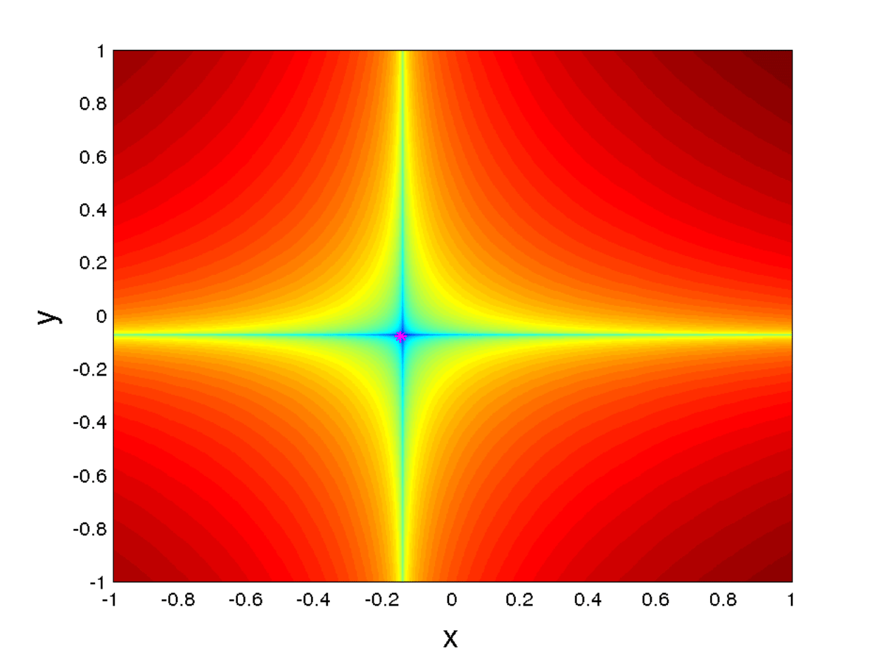
Fig. 46 Figure A) from [BILWM16] showing two different experiments representing contours of $MS_p$ for $p=0.1$ and $\tau=15$. The contours of $MS_p$ are computed on a 1200$\times$1200 points grid of initial conditions and the time step for integration of the vector field is chosen to be $\Delta t= 0.05$. The magenta colored point corresponds to the location of the stationary orbit for each experiment. The chosen parameters are $a_1 = a_2 = b_2 = 1$ and $b_1 = -1$.¶

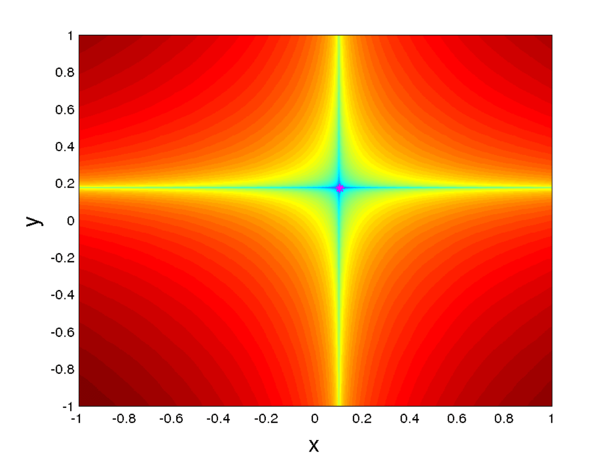
Fig. 47 Figure B) from [BILWM16] showing two different experiments representing contours of $MS_p$ for $p=0.1$ and $\tau=15$. The contours of $MS_p$ are computed on a 1200$\times$1200 points grid of initial conditions and the time step for integration of the vector field is chosen to be $\Delta t= 0.05$. The magenta colored point corresponds to the location of the stationary orbit for each experiment. The chosen parameters are $a_1 = a_2 = b_2 = 1$ and $b_1 = -1$.¶

Remark Due to the properties of Itô integrals, see for instance [Dua15], the components of the stationary orbit satisfy

(120)¶\[\mathbb{E} \left[ \tilde{x}(\omega ) \right] = \mathbb{E} \left[ - \int_{0}^{\infty}e^{-s}dW_{s}^{1} \right] = 0 \quad , \quad \mathbb{E} \left[ \tilde{y}(\omega ) \right] = \mathbb{E} \left[ \int_{-\infty}^{0}e^{s}dW_{s}^{2} \right] = 0\]

(121)¶\[\mathbb{V} \left[ \tilde{x}(\omega ) \right] = \mathbb{E} \left[ \tilde{x}(\omega )^{2} \right] = \mathbb{E} \left[ \int_{0}^{\infty}e^{-2s}ds \right] = \frac{1}{2} \quad , \quad \mathbb{V} \left[ \tilde{y}(\omega ) \right] = \mathbb{E} \left[ \tilde{y}(\omega )^{2} \right] = \mathbb{E} \left[ \int_{-\infty}^{0}e^{2s}ds \right] = \frac{1}{2}.\]

This means that the stationary orbit $(\tilde{x}(\omega ),\tilde{y}(\omega ))$ is highly probable to be located closed to the origin of coordinates $(0,0)$, and this feature is displayed in Fig. 47. This result gives more evidences and supports the similarities between the stochastic differential equation (90) and the deterministic analogue system $\lbrace \dot{x}=x, \hspace{0.1cm} \dot{y}=-y \rbrace$ whose only fixed point is $(0,0)$.

Therefore we can assert that the stochastic Lagrangian descriptor is a technique that provides a phase portrait representation of the dynamics generated by the noisy saddle equation (110). Next we apply this same technique to further examples.

The Stochastically forced Duffing Oscillator¶

Another classical problem is that of the Duffing oscillator. The deterministic version is given by

(122)¶\[\begin{equation} \label{eq:duffing_determ} \ddot{x} = \alpha \dot{x} + \beta x + \gamma x^3 + \epsilon \cos(t). \end{equation}\]

If $\epsilon = 0$ the Duffing equation becomes time-independent, meanwhile for $\epsilon \neq 0$ the oscillator is a time-dependent system, where $\alpha$ is the damping parameter, $\beta$ controls the rigidity of the system and $\gamma$ controls the size of the nonlinearity of the restoring force. The stochastically forced Duffing equation is studied in [datta01] and can be written as follows:

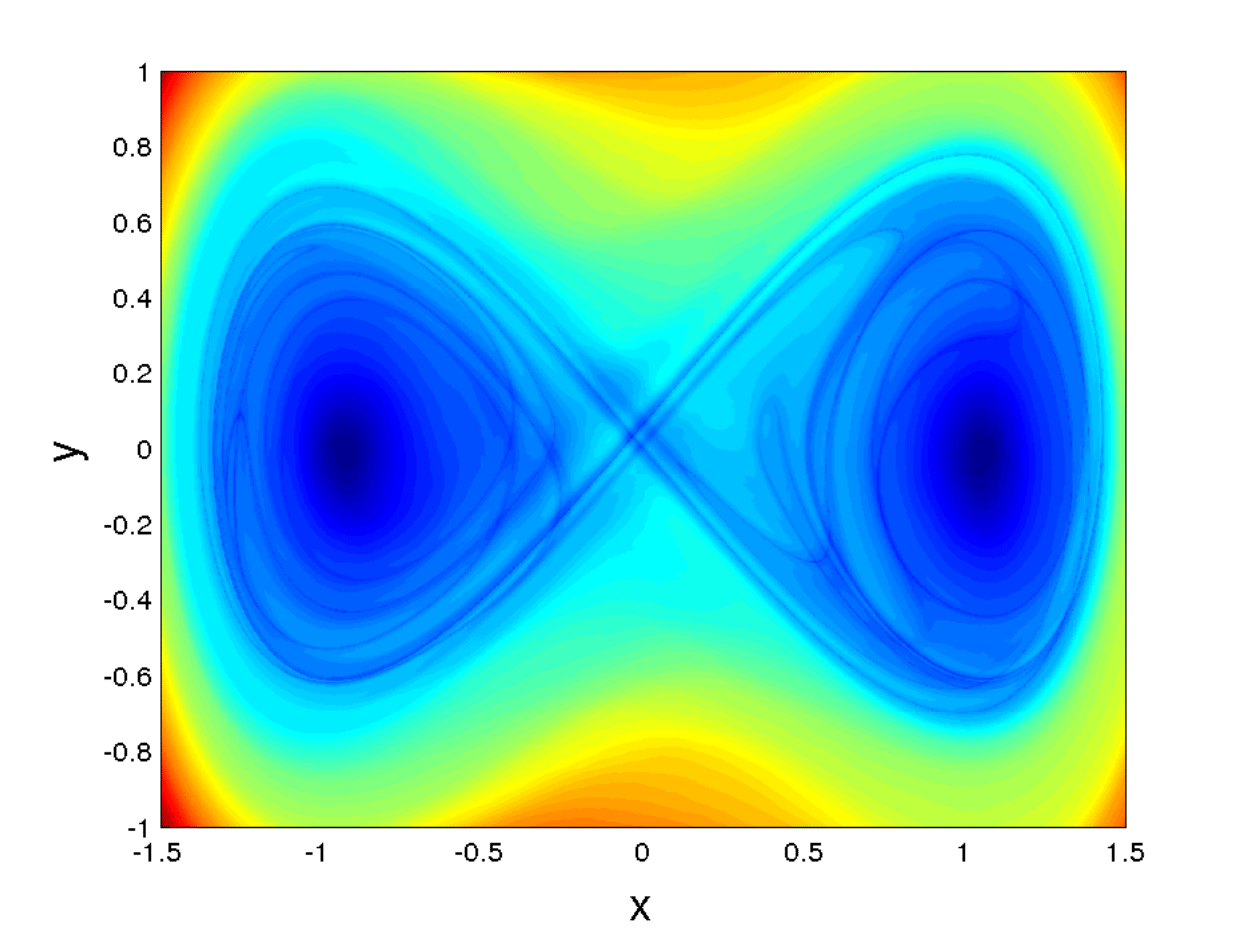
(123)¶\[\begin{split}\begin{equation} \begin{cases} dX_t = \alpha Y_t, \\ dY_t = (\beta X_t + \gamma X^3_t)dt + \epsilon dW_t. \end{cases} \end{equation}\end{split}\]

Fig. 48 Figure A) from [BILWM16] showing three different experiments representing $MS_p$ contours for $p=0.5$ over a grid of initial conditions.¶

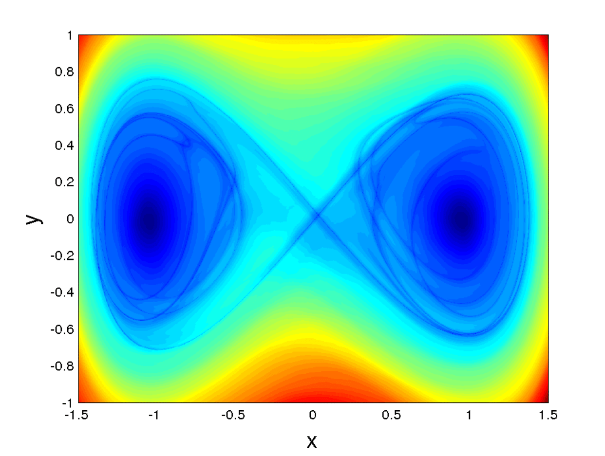
Fig. 49 Figure B) from [BILWM16] showing three different experiments representing $MS_p$ contours for $p=0.5$ over a grid of initial conditions.¶

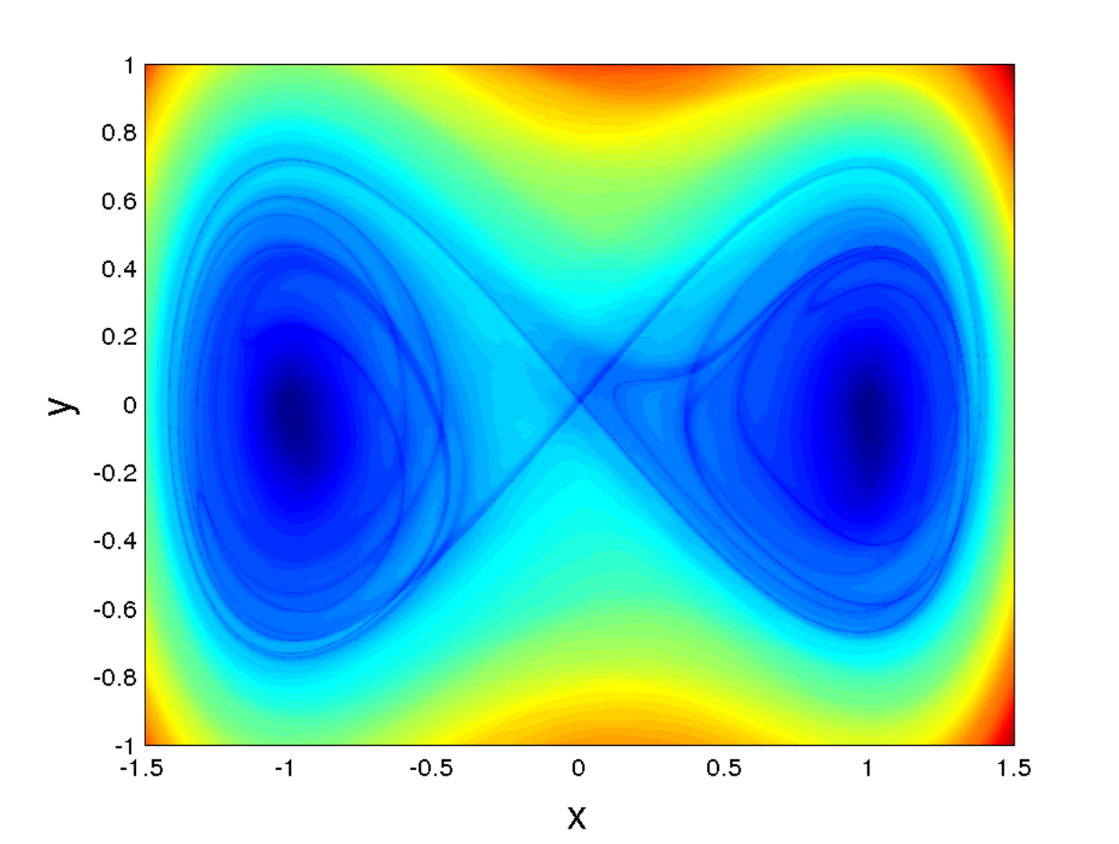
Fig. 50 Figure C) from [BILWM16] showing three different experiments representing $MS_p$ contours for $p=0.5$ over a grid of initial conditions. d) The last image corresponds to the $M_p$ function for equation (122) and $p=0.75$. All these pictures were computed for $\tau=15$, and over a $1200 \times 1200$ points grid. The time step for integration of the vector field was chosen to be $\Delta t = 0.05$.¶

Lagrangian Descriptors

The Method of Lagrangian Descriptors¶

Introduction¶

Lagrangian Descriptors versus Poincaré Maps¶

Autonomous Hamiltonian vector fields¶

Nonautonomous Hamiltonian vector fields¶

Formulations for Lagrangian Descriptors¶

The Arclength Definition¶

The \(p\)-norm Definition¶

Lagrangian Descriptors Based on the Classical Action¶

One Degree-of-Freedom Autonomous Hamiltonian Systems¶

\(n\) Degree-of-Freedom Autonomous Hamiltonian Systems¶

Variable Integration Time Lagrangian Descriptors¶

Examples¶

The Duffing Oscillator¶

The linear Hamiltonian saddle with 2 DoF¶

The Cubic Potential¶

The Hénon-Heiles Hamiltonian System¶

Stochastic Lagrangian Descriptors¶

Preliminary concepts¶

The stochastic Lagrangian descriptor¶

Numerical Simulation of the Stochastic Lagrangian Descriptor¶

The noisy saddle¶

The Stochastically forced Duffing Oscillator¶

References¶

References

- BILWM16(1,2,3,4,5,6)
Francisco Balibrea-Iniesta, Carlos Lopesino, Stephen Wiggins, and Ana M Mancho. Lagrangian descriptors for stochastic differential equations: a tool for revealing the phase portrait of stochastic dynamical systems. International Journal of Bifurcation and Chaos, 26(13):1630036, 2016.
- CDW16
Zhuan Cheng, Jinqiao Duan, and Liang Wang. Most probable dynamics of some nonlinear systems under noisy fluctuations. Communications in Nonlinear Science and Numerical Simulation, 30(1-3):108–114, 2016.
- CRO86
W.-L. Chien, H. Rising, and J. M. Ottino. Laminar mixing and chaotic mixing in several cavity flows. Journal of Fluid Mechanics, 170:355–377, 1986. doi:10.1017/S0022112086000927.
- CH15
Galen T Craven and Rigoberto Hernandez. Lagrangian descriptors of thermalized transition states on time-varying energy surfaces. Physical review letters, 115(14):148301, 2015.
- CH16
Galen T Craven and Rigoberto Hernandez. Deconstructing field-induced ketene isomerization through lagrangian descriptors. Physical Chemistry Chemical Physics, 18(5):4008–4018, 2016.
- CJH17
Galen T Craven, Andrej Junginger, and Rigoberto Hernandez. Lagrangian descriptors of driven chemical reaction manifolds. Physical Review E, 96(2):022222, 2017.
- CMMW19a
Jezabel Curbelo, Carlos R. Mechoso, Ana M. Mancho, and Stephen Wiggins. Lagrangian study of the final warming in the southern stratosphere during 2002: part i. the vortex splitting at upper levels. Climate Dynamics, 53(5):2779–2792, 2019. URL: https://doi.org/10.1007/s00382-019-04832-y, doi:10.1007/s00382-019-04832-y.
- CMMW19b
Jezabel Curbelo, Carlos R. Mechoso, Ana M. Mancho, and Stephen Wiggins. Lagrangian study of the final warming in the southern stratosphere during 2002: part ii. 3d structure. Climate Dynamics, 53(3):1277–1286, 2019. URL: https://doi.org/10.1007/s00382-019-04833-x, doi:10.1007/s00382-019-04833-x.
- dlCamaraMI+12
A. de la Cámara, A. M. Mancho, K. Ide, E. Serrano, and C.R. Mechoso. Routes of transport across the Antarctic polar vortex in the southern spring. J. Atmos. Sci., 69(2):753–767, 2012.
- dlCamaraMM+13
A. de la Cámara, R. Mechoso, A. M. Mancho, E. Serrano, and K. Ide. Isentropic transport within the Antarctic polar night vortex: Rossby wave breaking evidence and Lagrangian structures. J. Atmos. Sci., 70:2982–3001, 2013.
- DW17(1,2,3,4)
A. S. Demian and S. Wiggins. Detection of periodic orbits in Hamiltonian systems using Lagrangian descriptors. International Journal of Bifurcation and Chaos, 27(14):1750225, 2017. doi:10.1142/S021812741750225X.
- Dua15(1,2,3,4,5,6,7,8,9,10)
Jinqiao Duan. An introduction to stochastic dynamics. Volume 51. Cambridge University Press, 2015.
- FSB+19
Matthias Feldmaier, Philippe Schraft, Robin Bardakcioglu, Johannes Reiff, Melissa Lober, Martin Tschöpe, Andrej Junginger, Jörg Main, Thomas Bartsch, and Rigoberto Hernandez. Invariant manifolds and rate constants in driven chemical reactions. The Journal of Physical Chemistry B, 123(9):2070–2086, 2019. doi:10.1021/acs.jpcb.8b10541.
- GarciaGAW20
V. J. García-Garrido, M. Agaoglou, and S. Wiggins. Exploring isomerization dynamics on a potential energy surface with an index-2 saddle using lagrangian descriptors. Communications in Nonlinear Science and Numerical Simulation, 89:105331, 2020. doi:https://doi.org/10.1016/j.cnsns.2020.105331.
- GarciaGNW19
V. J. García-Garrido, S. Naik, and S. Wiggins. Tilting and squeezing: Phase space geometry of Hamiltonian saddle-node bifurcation and its influence on chemical reaction dynamics. arXiv preprint:1907.03322 (\it Under Review), 2019.
- GarciaGNW20(1,2,3)
V. J. García-Garrido, S. Naik, and S. Wiggins. Tilting and squeezing: Phase space geometry of Hamiltonian saddle-node bifurcation and its influence on chemical reaction dynamics. International Journal of Bifurcation and Chaos, 30(04):2030008, 2020. doi:10.1142/S0218127420300086.
- GGRM+16
V. J. Garcia-Garrido, A. Ramos, A. M. Mancho, J. Coca, and S. Wiggins. A dynamical systems perspective for a real-time response to a marine oil spill. Marine Pollution Bulletin., pages 1–10, 2016. doi:10.1016/j.marpolbul.2016.08.018.
- GarciaGCM+18
V. J. García-Garrido, J. Curbelo, A. M. Mancho, S. Wiggins, and C. R. Mechoso. The application of lagrangian descriptors to 3d vector fields. Regular and Chaotic Dynamics, 23(5):551–568, 2018. doi:10.1134/S1560354718050052.
- GPS02
Herbert Goldstein, Charles Poole, and John Safko. Classical mechanics. 2002.
- HenonH64
M. Hénon and C. Heiles. The Applicability of the Third Integral of Motion: Some Numerical Experiments. Astronom. J., 69:73–79, 1964. doi:10.1086/109234.
- JDF+17(1,2)
Andrej Junginger, Lennart Duvenbeck, Matthias Feldmaier, Jörg Main, Günter Wunner, and Rigoberto Hernandez. Chemical dynamics between wells across a time-dependent barrier: self-similarity in the lagrangian descriptor and reactive basins. The Journal of chemical physics, 147(6):064101, 2017.
- KGarciaGW20
M. Katsanikas, V. J. García-Garrido, and S. Wiggins. The dynamical matching mechanism in phase space for caldera-type potential energy surfaces. Chemical Physics Letters, 743:137199, 2020. doi:https://doi.org/10.1016/j.cplett.2020.137199.
- KP13
Peter E Kloeden and Eckhard Platen. Numerical solution of stochastic differential equations. Volume 23. Springer Science & Business Media, 2013.
- KR11
Peter E Kloeden and Martin Rasmussen. Nonautonomous dynamical systems. Number 176. American Mathematical Soc., 2011.
- KrajvnakEW19
V. Krajňák, G.S. Ezra, and S. Wiggins. Roaming at Constant Kinetic Energy: Chesnavich’s Model and the Hamiltonian Isokinetic Thermostat. Regul. Chaot. Dyn., 24:615–627, 2019. doi:https://doi.org/10.1134/S1560354719060030.
- LL13
Lev Davidovič Landau and Evgenii Mikhailovich Lifshitz. Mechanics and electrodynamics. Elsevier, 2013.
- LBIGarciaG+17(1,2)
C. Lopesino, F. Balibrea-Iniesta, V. J. García-Garrido, S. Wiggins, and A. M. Mancho. A theoretical framework for lagrangian descriptors. International Journal of Bifurcation and Chaos, 27(01):1730001, 2017. doi:10.1142/S0218127417300014.
- LBIWMancho15
C. Lopesino, F. Balibrea-Iniesta, S. Wiggins, and A. M. Mancho. Lagrangian descriptors for two dimensional, area preserving autonomous and nonautonomous maps. Communications in Nonlinear Science and Numerical Simulation, 27(1-3):40–51, 2015. doi:10.1016/j.cnsns.2015.02.022.
- MM09
J. A. J. Madrid and A. M. Mancho. Distinguished trajectories in time dependent vector fields. Chaos, 19:013111, 2009.
- MWCM13(1,2)
A. M. Mancho, S. Wiggins, J. Curbelo, and C. Mendoza. Lagrangian descriptors: a method for revealing phase space structures of general time dependent dynamical systems. Communications in Nonlinear Science and Numerical Simulation, 18(12):3530–3557, 2013.
- MM10
Carolina Mendoza and Ana M. Mancho. Hidden geometry of ocean flows. Phys. Rev. Lett., 105:038501, 2010. doi:10.1103/PhysRevLett.105.038501.
- MW20a
Francisco Gonzalez Montoya and Stephen Wiggins. Revealing roaming on the double morse potential energy surface with lagrangian descriptors. Journal of Physics A: Mathematical and Theoretical, 53(23):235702, 2020. URL: https://doi.org/10.1088/1751-8121/ab8b75, doi:10.1088/1751-8121/ab8b75.
- MW20b
Francisco Gonzalez Montoya and Stephen Wiggins. The phase space structure and the escape time dynamics in a van der waals model for exothermic reactions. 2020. arXiv:2006.15611.
- NGarciaGW19(1,2,3,4)
Shibabrat Naik, Víctor J. García-Garrido, and Stephen Wiggins. Finding NHIM: identifying high dimensional phase space structures in reaction dynamics using Lagrangian descriptors. Communications in Nonlinear Science and Numerical Simulation, 79:104907, 2019. doi:10.1016/j.cnsns.2019.104907.
- NW19(1,2,3)
Shibabrat Naik and Stephen Wiggins. Finding normally hyperbolic invariant manifolds in two and three degrees of freedom with Hénon-Heiles type potential. Phys. Rev. E, 100:022204, 2019. doi:10.1103/PhysRevE.100.022204.
- NW20
Shibabrat Naik and Stephen Wiggins. Detecting reactive islands in a system-bath model of isomerization. Phys. Chem. Chem. Phys., 2020. doi:10.1039/D0CP01362E.
- Oks03
Bernt Oksendal. Stochastic Differential Equations: An Introduction with Applications. Universitext. Springer-Verlag Berlin Heidelberg, 6 edition, 2003.
- Poincare90
Henri Poincaré. Sur le problème des trois corps et les équations de dynamique. Acta Mathica, 13:1–270, 1890.
- RGarciaGM+18
A. G. Ramos, V. J. García-Garrido, A. M. Mancho, S. Wiggins, J. Coca, S. Glenn, O. Schofield, J. Kohut, D. Aragon, J. Kerfoot, T. Haskins, T. Miles, C. Haldeman, N. Strandskov, B. Allsup, C. Jones, and J. Shapiro. Lagrangian coherent structure assisted path planning for transoceanic autonomous underwater vehicle missions. Scientfic Reports, 4:4575, 2018. doi:10.1038/s41598-018-23028-8.
- RBB19
F Revuelta, RM Benito, and F Borondo. Unveiling the chaotic structure in phase space of molecular systems using lagrangian descriptors. Physical Review E, 99(3):032221, 2019.